Turning quantum nodes into Torch Layers

Author: Tom Bromley — Posted: 02 November 2020. Last updated: 28 January 2021.

Creating neural networks in PyTorch is easy using the nn module. Models are constructed from elementary layers and can be trained using the PyTorch API. For example, the following code defines a two-layer network that could be used for binary classification:

import torch

layer_1 = torch.nn.Linear(2, 2)
layer_2 = torch.nn.Linear(2, 2)
softmax = torch.nn.Softmax(dim=1)

layers = [layer_1, layer_2, softmax]
model = torch.nn.Sequential(*layers)

What if we want to add a quantum layer to our model? This is possible in PennyLane: QNodes can be converted into torch.nn layers and combined with the wide range of built-in classical layers to create truly hybrid models. This tutorial will guide you through a simple example to show you how it’s done!

Note

A similar demo explaining how to turn quantum nodes into Keras layers is also available.

Fixing the dataset and problem

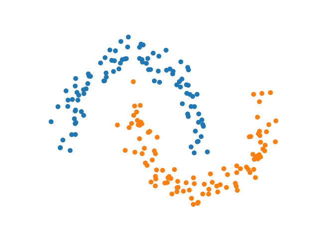
Let us begin by choosing a simple dataset and problem to allow us to focus on how the hybrid model is constructed. Our objective is to classify points generated from scikit-learn’s binary-class make_moons() dataset:

import matplotlib.pyplot as plt
import numpy as np
from sklearn.datasets import make_moons

# Set random seeds
torch.manual_seed(42)
np.random.seed(42)

X, y = make_moons(n_samples=200, noise=0.1)
y_ = torch.unsqueeze(torch.tensor(y), 1)  # used for one-hot encoded labels
y_hot = torch.scatter(torch.zeros((200, 2)), 1, y_, 1)

c = ["#1f77b4" if y_ == 0 else "#ff7f0e" for y_ in y]  # colours for each class
plt.axis("off")
plt.scatter(X[:, 0], X[:, 1], c=c)
plt.show()

Defining a QNode

Our next step is to define the QNode that we want to interface with torch.nn. Any combination of device, operations and measurements that is valid in PennyLane can be used to compose the QNode. However, the QNode arguments must satisfy additional conditions including having an argument called inputs. All other arguments must be arrays or tensors and are treated as trainable weights in the model. We fix a two-qubit QNode using the default.qubit simulator and operations from the templates module.

import pennylane as qml

n_qubits = 2
dev = qml.device("default.qubit", wires=n_qubits)

@qml.qnode(dev)
def qnode(inputs, weights):
    qml.AngleEmbedding(inputs, wires=range(n_qubits))
    qml.BasicEntanglerLayers(weights, wires=range(n_qubits))
    return [qml.expval(qml.PauliZ(wires=i)) for i in range(n_qubits)]

Interfacing with Torch

With the QNode defined, we are ready to interface with torch.nn. This is achieved using the TorchLayer class of the qnn module, which converts the QNode to the elementary building block of torch.nn: a layer. We shall see in the following how the resultant layer can be combined with other well-known neural network layers to form a hybrid model.

We must first define the weight_shapes dictionary. Recall that all of the arguments of the QNode (except the one named inputs) are treated as trainable weights. For the QNode to be successfully converted to a layer in torch.nn, we need to provide the details of the shape of each trainable weight for them to be initialized. The weight_shapes dictionary maps from the argument names of the QNode to corresponding shapes:

n_layers = 6
weight_shapes = {"weights": (n_layers, n_qubits)}

In our example, the weights argument of the QNode is trainable and has shape given by (n_layers, n_qubits), which is passed to BasicEntanglerLayers().

Now that weight_shapes is defined, it is easy to then convert the QNode:

qlayer = qml.qnn.TorchLayer(qnode, weight_shapes)

With this done, the QNode can now be treated just like any other torch.nn layer and we can proceed using the familiar Torch workflow.

Creating a hybrid model

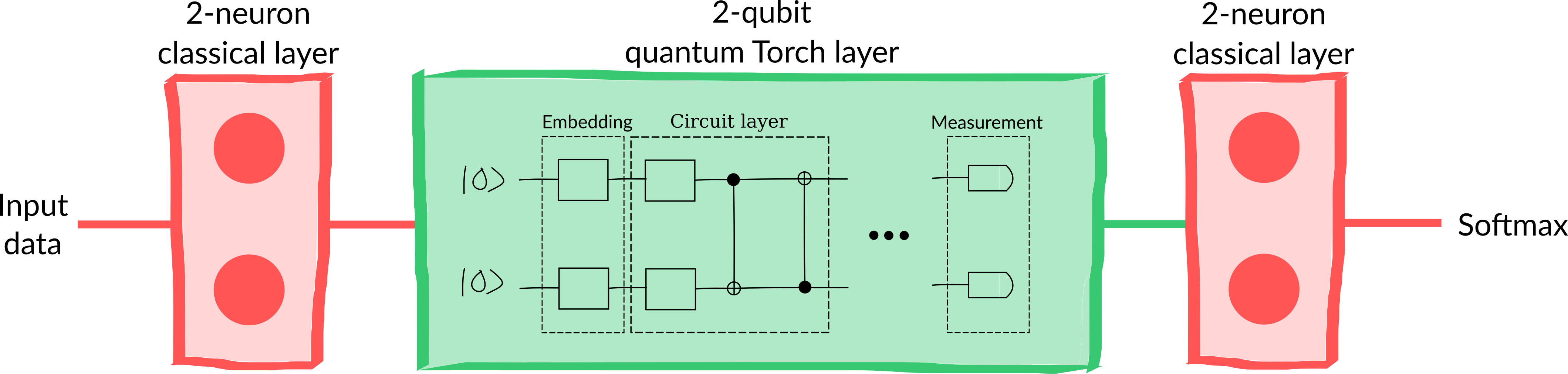
Let’s create a basic three-layered hybrid model consisting of:

1. a 2-neuron fully connected classical layer

2. our 2-qubit QNode converted into a layer

3. another 2-neuron fully connected classical layer

4. a softmax activation to convert to a probability vector

A diagram of the model can be seen in the figure below.

We can construct the model using the Sequential API:

clayer_1 = torch.nn.Linear(2, 2)
clayer_2 = torch.nn.Linear(2, 2)
softmax = torch.nn.Softmax(dim=1)
layers = [clayer_1, qlayer, clayer_2, softmax]
model = torch.nn.Sequential(*layers)

Training the model

We can now train our hybrid model on the classification dataset using the usual Torch approach. We’ll use the standard SGD optimizer and the mean absolute error loss function:

opt = torch.optim.SGD(model.parameters(), lr=0.2)
loss = torch.nn.L1Loss()

Note that there are more advanced combinations of optimizer and loss function, but here we are focusing on the basics.

The model is now ready to be trained!

X = torch.tensor(X, requires_grad=True).float()
y_hot = y_hot.float()

batch_size = 5
batches = 200 // batch_size

data_loader = torch.utils.data.DataLoader(
    list(zip(X, y_hot)), batch_size=5, shuffle=True, drop_last=True
)

epochs = 6

for epoch in range(epochs):

    running_loss = 0

    for xs, ys in data_loader:
        opt.zero_grad()

        loss_evaluated = loss(model(xs), ys)
        loss_evaluated.backward()

        opt.step()

        running_loss += loss_evaluated

    avg_loss = running_loss / batches
    print("Average loss over epoch {}: {:.4f}".format(epoch + 1, avg_loss))

y_pred = model(X)
predictions = torch.argmax(y_pred, axis=1).detach().numpy()

correct = [1 if p == p_true else 0 for p, p_true in zip(predictions, y)]
accuracy = sum(correct) / len(correct)
print(f"Accuracy: {accuracy * 100}%")

Out:

Average loss over epoch 1: 0.4943
Average loss over epoch 2: 0.4226
Average loss over epoch 3: 0.2847
Average loss over epoch 4: 0.2121
Average loss over epoch 5: 0.1845
Average loss over epoch 6: 0.1666
Accuracy: 85.5%

How did we do? The model looks to have successfully trained and the accuracy is reasonably high. In practice, we would aim to push the accuracy higher by thinking carefully about the model design and the choice of hyperparameters such as the learning rate.

Creating non-sequential models

The model we created above was composed of a sequence of classical and quantum layers. This type of model is very common and is suitable in a lot of situations. However, in some cases we may want a greater degree of control over how the model is constructed, for example when we have multiple inputs and outputs or when we want to distribute the output of one layer into multiple subsequent layers.

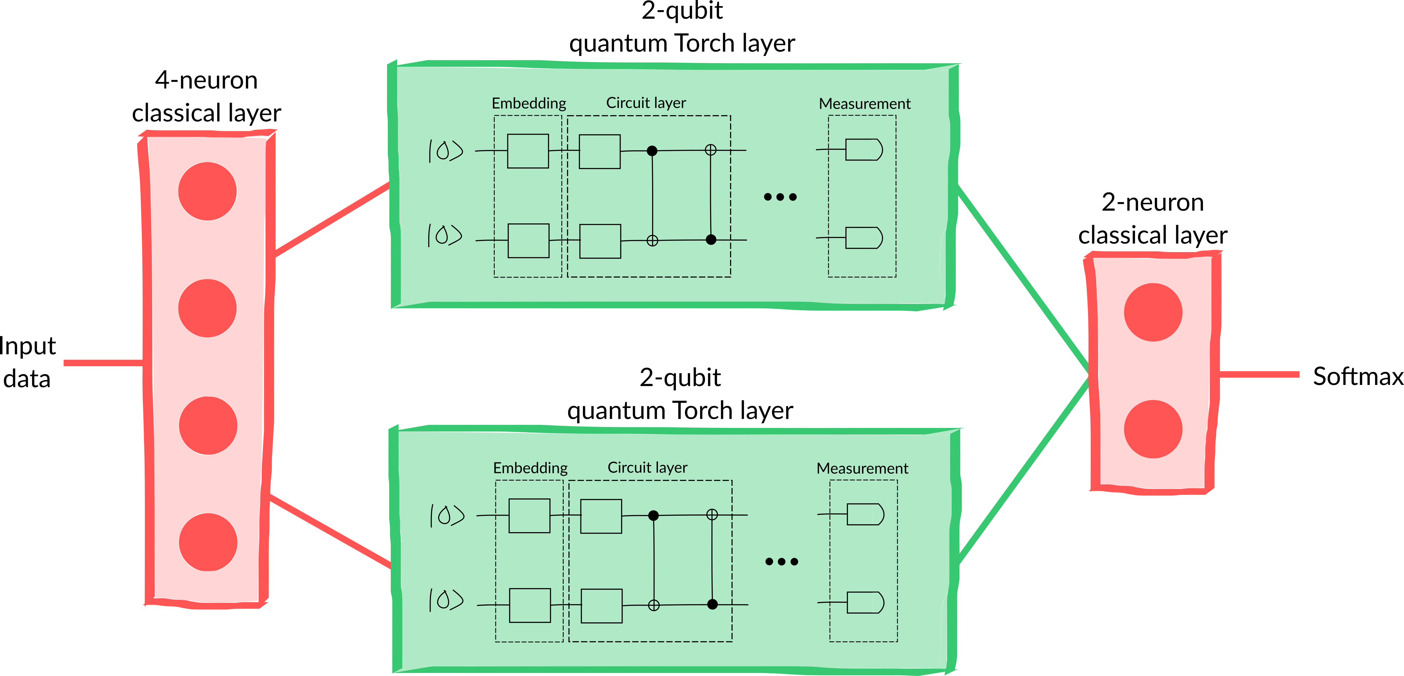
Suppose we want to make a hybrid model consisting of:

1. a 4-neuron fully connected classical layer

2. a 2-qubit quantum layer connected to the first two neurons of the previous classical layer

3. a 2-qubit quantum layer connected to the second two neurons of the previous classical layer

4. a 2-neuron fully connected classical layer which takes a 4-dimensional input from the combination of the previous quantum layers

5. a softmax activation to convert to a probability vector

A diagram of the model can be seen in the figure below.

This model can also be constructed by creating a new class that inherits from the torch.nn Module and overriding the forward() method:

class HybridModel(torch.nn.Module):
    def __init__(self):
        super().__init__()
        self.clayer_1 = torch.nn.Linear(2, 4)
        self.qlayer_1 = qml.qnn.TorchLayer(qnode, weight_shapes)
        self.qlayer_2 = qml.qnn.TorchLayer(qnode, weight_shapes)
        self.clayer_2 = torch.nn.Linear(4, 2)
        self.softmax = torch.nn.Softmax(dim=1)

    def forward(self, x):
        x = self.clayer_1(x)
        x_1, x_2 = torch.split(x, 2, dim=1)
        x_1 = self.qlayer_1(x_1)
        x_2 = self.qlayer_2(x_2)
        x = torch.cat([x_1, x_2], axis=1)
        x = self.clayer_2(x)
        return self.softmax(x)

model = HybridModel()

As a final step, let’s train the model to check if it’s working:

opt = torch.optim.SGD(model.parameters(), lr=0.2)
epochs = 6

for epoch in range(epochs):

    running_loss = 0

    for xs, ys in data_loader:
        opt.zero_grad()

        loss_evaluated = loss(model(xs), ys)
        loss_evaluated.backward()

        opt.step()

        running_loss += loss_evaluated

    avg_loss = running_loss / batches
    print("Average loss over epoch {}: {:.4f}".format(epoch + 1, avg_loss))

y_pred = model(X)
predictions = torch.argmax(y_pred, axis=1).detach().numpy()

correct = [1 if p == p_true else 0 for p, p_true in zip(predictions, y)]
accuracy = sum(correct) / len(correct)
print(f"Accuracy: {accuracy * 100}%")

Out:

Average loss over epoch 1: 0.4333
Average loss over epoch 2: 0.2811
Average loss over epoch 3: 0.2164
Average loss over epoch 4: 0.1909
Average loss over epoch 5: 0.1704
Average loss over epoch 6: 0.1639
Accuracy: 85.5%

Great! We’ve mastered the basics of constructing hybrid classical-quantum models using PennyLane and Torch. Can you think of any interesting hybrid models to construct? How do they perform on realistic datasets?

About the author

Thomas Bromley

Thomas is a quantum scientist working at Xanadu. His work is focused on developing software to execute quantum algorithms on simulators and hardware.

demos/tutorial_qnn_module_torch

 

Download Python script

 

Download Notebook

 

View on GitHub