Quantum detection of time series anomalies

Authors: Jack Stephen Baker, Santosh Kumar Radha — Posted: 7 February 2023.

Systems producing observable characteristics which evolve with time are almost everywhere we look. The temperature changes as day turns to night, stock markets fluctuate and the bacteria colony living in the coffee cup to your right, which you promised you would clean yesterday, is slowly growing (seriously, clean it). In many situations, it is important to know when these systems start behaving abnormally. For example, if the pressure inside a nuclear fission reactor starts violently fluctuating, you may wish to be alerted of that. The task of identifying such temporally abnormal behaviour is known as time series anomaly detection and is well known in machine learning circles.

In this tutorial, we take a stab at time series anomaly detection using the Quantum Variational Rewinding algorithm, or QVR, proposed by Baker, Horowitz, Radha et. al (2022) 1 — a quantum machine learning algorithm for gate model quantum computers. QVR leverages the power of unitary time evolution/devolution operators to learn a model of normal behaviour for time series data. Given a new (i.e., unseen in training) time series, the normal model produces a value that, beyond a threshold, defines anomalous behaviour. In this tutorial, we’ll be showing you how all of this works, combining elements from Covalent, Pennylane and PyTorch.

Before getting into the technical details of the algorithm, let’s get a high-level overview with the help of the cartoon below.

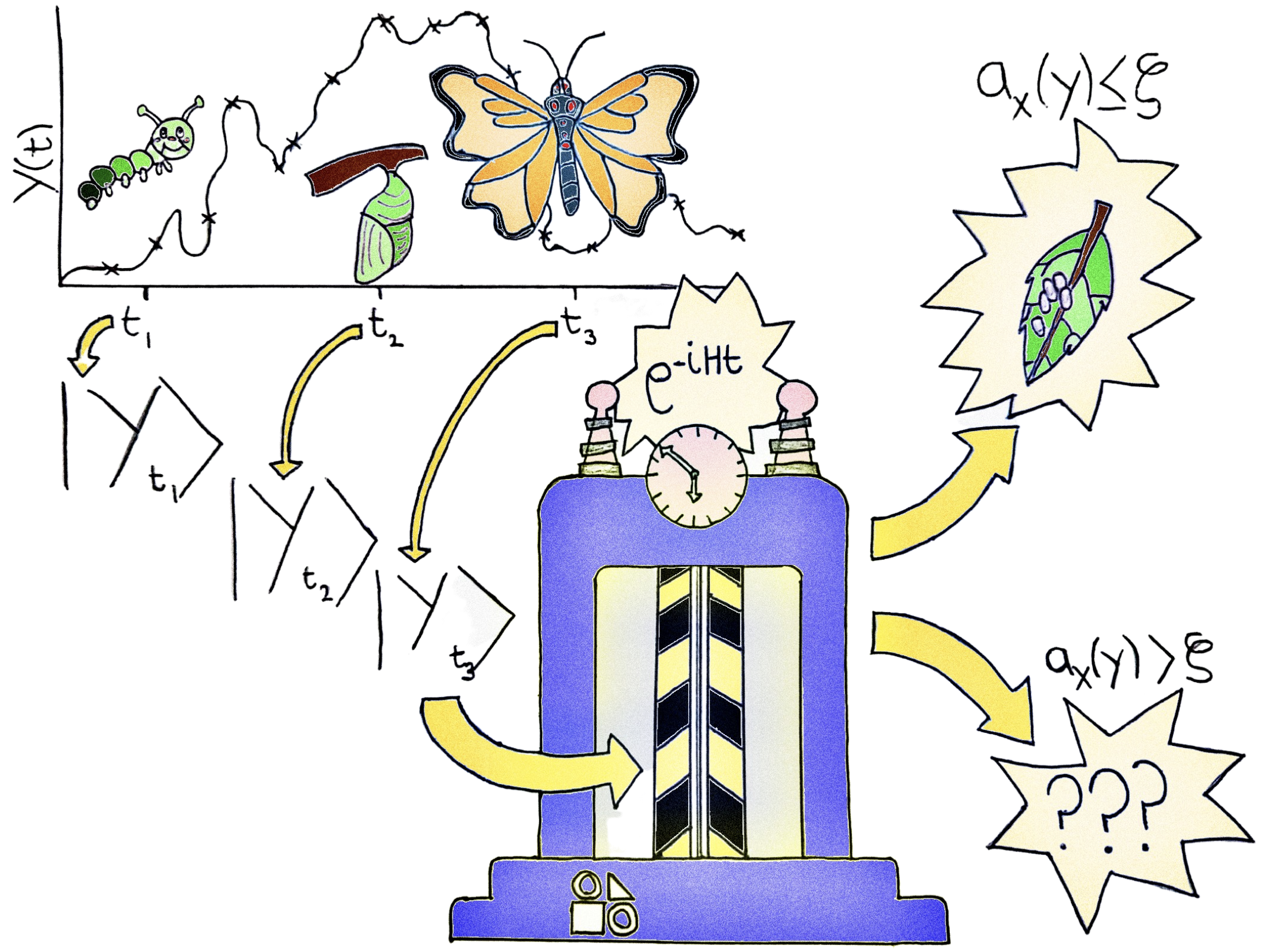
Going left-to-right, a time series is sampled at three points in time, corresponding to different stages in the life cycle of a butterfly: a catepillar, a chrysalis and a butterfly. This information is then encoded into quantum states and passed to a time machine which time devolves the states as generated by a learnt Hamiltonian operator (in practice, there is a distribution of such operators). After the devolved state is measured, the time series is recognized as normal if the average measurement is smaller than a given threshold and anomalous if the threshold is exceeded. In the first case, the time series is considered rewindable, correctly recovering the initial condition for the life cycle of a butterfly: eggs on a leaf. In the second case, the output is unrecognizable.

This will all make more sense once we delve into the math a little. Let’s do it!

Background

To begin, let’s quickly recount the data that QVR handles: time series. A general time series \(\boldsymbol{y}\) can be described as a sequence of \(p\)-many observations of a process/system arranged in chronological order, where \(p\) is a positive integer:

\[\boldsymbol{y} := (\boldsymbol{y}_t: t \in T), \quad T := (t_l: l \in \mathbb{Z}^{+}_{\leq p}).\]

In the simple and didactic case treated in this tutorial, \(\boldsymbol{y}\) is univariate (i.e, is a one-dimensional time series), so bold-face for \(\boldsymbol{y}\) is dropped from this point onwards. Also, we take \(y_t \in \mathbb{R}\) and \(t_l \in \mathbb{R}_{>0}\).

The goal of QVR and many other (classical) machine learning algorithms for time series anomaly detection is to determine a suitable anomaly score function \(a_{X}\), where \(X\) is a training dataset of normal time series instances \(x \in X\) (\(x\) is defined analogously to \(y\) in the above), from which the anomaly score function was learnt. When passed a general time series \(y\), this function produces a real number: \(a_X(y) \in \mathbb{R}\). The goal is to have \(a_X(x) \approx 0\), for all \(x \in X\). Then, for an unseen time series \(y\) and a threshold \(\zeta \in \mathbb{R}\), the series is said to be anomalous should \(a_X(y) > \zeta,\) and normal otherwise. We show a strategy for setting \(\zeta\) later in this tutorial.

The first step for doing all of this quantumly is to generate a sequence \(\mathcal{S} := (|x_{t} \rangle: t \in T)\) of \(n\)-qubit quantum states corresponding to a classical time series instance in the training set. Now, we suppose that each \(|x_t \rangle\) is a quantum state evolved to a time \(t\), as generated by an unknown embedding Hamiltonian \(H_E\). That is, each element of \(\mathcal{S}\) is defined by \(|x_t \rangle = e^{-iH_E(x_t)}|0\rangle^{\otimes n} = U(x_t)|0\rangle^{\otimes n}\) for an embedding unitary operator \(U(x_t)\) implementing a quantum feature map (see the Pennylane embedding templates for efficient quantum circuits for doing so). Next, we operate on each \(|x_t\rangle\) with a parameterized \(e^{-iH(\boldsymbol{\alpha}, \boldsymbol{\gamma})t}\) operator to prepare the states

\[|x_t, \boldsymbol{\alpha}, \boldsymbol{\gamma}\rangle := e^{-iH(\boldsymbol{\alpha}, \boldsymbol{\gamma})t}|x_t\rangle,\]

where we write \(e^{-iH(\boldsymbol{\alpha}, \boldsymbol{\gamma})t}\) as an eigendecomposition

\[V_t(\boldsymbol{\alpha}, \boldsymbol{\gamma}) := W^{\dagger}(\boldsymbol{\alpha})D(\boldsymbol{\gamma}, t)W(\boldsymbol{\alpha}) = e^{-iH(\boldsymbol{\alpha}, \boldsymbol{\gamma})t}.\]

Here, the unitary matrix of eigenvectors \(W(\boldsymbol{\alpha})\) is parametrized by \(\boldsymbol{\alpha}\) and the unitary diagonalization \(D(\boldsymbol{\gamma}, t)\) is parametrized by \(\boldsymbol{\gamma}.\) Both can be implemented efficiently using parameterized quantum circuits. The above equality with \(e^{-iH(\boldsymbol{\alpha}, \boldsymbol{\gamma})t}\) is a consequence of Stone’s theorem for strongly continuous one-parameter unitary groups 2.

We now ask the question: What condition is required for \(|x_t, \boldsymbol{\alpha}, \boldsymbol{\gamma} \rangle = |0 \rangle^{\otimes n}\) for all time? To answer this, we impose \(P(|0\rangle^{\otimes n}) = |\langle 0|^{\otimes n}|x_t, \boldsymbol{\alpha}, \boldsymbol{\gamma} \rangle|^2 = 1.\) Playing with the algebra a little, we find that the following condition must be satisfied for all \(t\):

\[\langle 0|^{\otimes n}e^{-iH(\boldsymbol{\alpha}, \boldsymbol{\gamma})t}e^{-iH_E(x_t)}|0\rangle^{\otimes n} = 1 \iff H(\boldsymbol{\alpha}, \boldsymbol{\gamma})t = -H_E(x_t).\]

In other words, for the above to be true, the parameterized unitary operator \(V_t(\boldsymbol{\alpha}, \boldsymbol{\gamma})\) should be able to reverse or rewind \(|x_t\rangle\) to its initial state \(|0\rangle^{\otimes n}\) before the embedding unitary operator \(U(x_t)\) was applied.

We are nearly there! Because it is reasonable to expect that a single Hamiltonian will not be able to successfully rewind every \(x \in X\) (in fact, this is impossible to do if each \(x\) is unique, which is usually true), we consider the average effect of many Hamiltonians generated by drawing \(\boldsymbol{\gamma}\) from a normal distribution \(\mathcal{N}(\mu, \sigma)\) with mean \(\mu\) and standard deviation \(\sigma\):

\[F(\boldsymbol{\phi}, x_t) := \mathop{\mathbb{E}_{\boldsymbol{\gamma} \sim \mathcal{N}(\mu, \sigma)}}\left[\langle 0|^{\otimes n} |x_t, \boldsymbol{\alpha}, \boldsymbol{\gamma}\rangle \right], \quad \boldsymbol{\phi} = [\boldsymbol{\alpha}, \mu, \sigma].\]

The goal is for the function \(F\) defined above to be as close to \(1\) as possible, for all \(x \in X\) and \(t \in T.\) With this in mind, we can define the loss function to minimize as the mean square error regularized by a penalty function \(P_{\tau}(\sigma)\) with a single hyperparameter \(\tau\):

\[\mathcal{L(\boldsymbol{\phi})} = \frac{1}{2|X||T|}\sum_{x \in X} \sum_{t \in T}[1 - F(\boldsymbol{\phi}, x_t)]^2 + P_{\tau}(\sigma).\]

We will show the exact form of \(P_{\tau}(\sigma)\) later. The general purpose of the penalty function is to penalize large values of \(\sigma\) (justification for this is given in the Supplement of 1). After approximately finding the argument \(\boldsymbol{\phi}^{\star}\) that minimizes the loss function (found using a classical optimization routine), we finally arrive at a definition for our anomaly score function \(a_X(y)\)

\[a_X(y) = \frac{1}{|T|}\sum_{t \in T}[1 - F(\boldsymbol{\phi}^{\star}, y_t)]^2.\]

It may now be apparent that we have implemented a clustering algorithm! That is, our model \(F\) was trained such that normal time series \(x \in X\) produce \(F(\boldsymbol{\phi}^{\star}, x_t)\) clustered about a center at \(1\). Given a new time series \(y\), should \(F(\boldsymbol{\phi}^{\star}, y_t)\) venture far from the normal center at \(1\), we are observing anomalous behaviour!

Take the time now to have another look at the cartoon at the start of this tutorial. Hopefully things should start making sense now.

Now with our algorithm defined, let’s stitch this all together: enter Covalent.

Covalent: heterogeneous workflow orchestration

Presently, many QML algorithms are heterogeneous in nature. This means that they require computational resources from both classical and quantum computing. Covalent is a tool that can be used to manage their interaction by sending different tasks to different computational resources and stitching them together as a workflow. While you will be introduced to other concepts in Covalent throughout this tutorial, we define two key components to begin with.

1. Electrons. Decorate regular Python functions with @ct.electron to desginate a task. These are the atoms of a computation.

2. Lattices. Decorate a regular Python function with @ct.lattice to designate a workflow. These contain electrons stitched together to do something useful.

   Different electrons can be run remotely on different hardware and multiple computational paridigms (classical, quantum, etc.: see the Covalent executors). In this tutorial, however, to keep things simple, tasks are run on a local Dask cluster, which provides (among other things) auto-parallelization.

Now is a good time to import Covalent and launch the Covalent server!

import covalent as ct
import os
import time

# Set up Covalent server
os.environ["COVALENT_SERVER_IFACE_ANY"] = "1"
os.system("covalent start")
# If you run into any out-of-memory issues with Dask when running this notebook,
# Try reducing the number of workers and making a specific memory request. I.e.:
# os.system("covalent start -m "2GiB" -n 2")
# try covalent –help for more info
time.sleep(2)  # give the Dask cluster some time to launch

Generating univariate synthetic time series

In this tutorial, we shall deal with a simple and didactic example. Normal time series instances are chosen to be noisy low-amplitude signals normally distributed about the origin. In our case, \(x_t \sim \mathcal{N}(0, 0.1)\). Series we deem to be anomalous are the same but with randomly inserted spikes with random durations and amplitudes.

Let’s make a @ct.electron to generate each of these synthetic time series sets. For this, we’ll need to import Torch. We’ll also set the default tensor type and pick a random seed for the whole tutorial for reproducibility.

import torch

# Seed Torch for reproducibility and set default tensor type
GLOBAL_SEED = 1989
torch.manual_seed(GLOBAL_SEED)
torch.set_default_tensor_type(torch.DoubleTensor)


@ct.electron
def generate_normal_time_series_set(
    p: int, num_series: int, noise_amp: float, t_init: float, t_end: float, seed: int = GLOBAL_SEED
) -> tuple:
    """Generate a normal time series data set where each of the p elements
    is drawn from a normal distribution x_t ~ N(0, noise_amp).
    """
    torch.manual_seed(seed)
    X = torch.normal(0, noise_amp, (num_series, p))
    T = torch.linspace(t_init, t_end, p)
    return X, T


@ct.electron
def generate_anomalous_time_series_set(
    p: int,
    num_series: int,
    noise_amp: float,
    spike_amp: float,
    max_duration: int,
    t_init: float,
    t_end: float,
    seed: int = GLOBAL_SEED,
) -> tuple:
    """Generate an anomalous time series data set where the p elements of each sequence are
    from a normal distribution x_t ~ N(0, noise_amp). Then,
    anomalous spikes of random amplitudes and durations are inserted.
    """
    torch.manual_seed(seed)
    Y = torch.normal(0, noise_amp, (num_series, p))
    for y in Y:
        # 5–10 spikes allowed
        spike_num = torch.randint(low=5, high=10, size=())
        durations = torch.randint(low=1, high=max_duration, size=(spike_num,))
        spike_start_idxs = torch.randperm(p - max_duration)[:spike_num]
        for start_idx, duration in zip(spike_start_idxs, durations):
            y[start_idx : start_idx + duration] += torch.normal(0.0, spike_amp, (duration,))
    T = torch.linspace(t_init, t_end, p)
    return Y, T

Let’s do a quick sanity check and plot a couple of these series. Despite the above function’s @ct.electron decorators, these can still be used as normal Python functions without using the Covalent server. This is useful for quick checks like this:

import matplotlib.pyplot as plt

X_norm, T_norm = generate_normal_time_series_set(25, 25, 0.1, 0.1, 2 * torch.pi)
Y_anom, T_anom = generate_anomalous_time_series_set(25, 25, 0.1, 0.4, 5, 0, 2 * torch.pi)

plt.figure()
plt.plot(T_norm, X_norm[0], label="Normal")
plt.plot(T_anom, Y_anom[1], label="Anomalous")
plt.ylabel("$y(t)$")
plt.xlabel("t")
plt.grid()
leg = plt.legend()

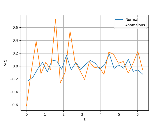
Taking a look at the above, the generated series are what we wanted. We have a simple human-parsable notion of what it is for a time series to be anomalous (big spikes). Of course, we don’t need a complicated algorithm to be able to detect such anomalies but this is just a didactic example remember!

Like many machine learning algorithms, training is done in mini-batches. Examining the form of the loss function \(\mathcal{L}(\boldsymbol{\phi})\), we can see that time series are atomized. In other words, each term in the mean square error is for a given \(x_t\) and not measured against the entire series \(x\). This allows us to break down the training set \(X\) into time-series-independent chunks. Here’s an electron to do that:

@ct.electron
def make_atomized_training_set(X: torch.Tensor, T: torch.Tensor) -> list:
    """Convert input time series data provided in a two-dimensional tensor format
    to atomized tuple chunks: (xt, t).
    """
    X_flat = torch.flatten(X)
    T_flat = T.repeat(X.size()[0])
    atomized = [(xt, t) for xt, t in zip(X_flat, T_flat)]
    return atomized

We now wish to pass this to a cycled torch.utils.data.DataLoader. However, this object is not pickleable, which is a requirement of electrons in Covalent. We therefore use the below helper class to create a pickleable version.

from collections.abc import Iterator


class DataGetter:
    """A pickleable mock-up of a Python iterator on a torch.utils.Dataloader.
    Provide a dataset X and the resulting object O will allow you to use next(O).
    """

    def __init__(self, X: torch.Tensor, batch_size: int, seed: int = GLOBAL_SEED) -> None:
        """Calls the _init_data method on intialization of a DataGetter object."""
        torch.manual_seed(seed)
        self.X = X
        self.batch_size = batch_size
        self.data = []
        self._init_data(
            iter(torch.utils.data.DataLoader(self.X, batch_size=self.batch_size, shuffle=True))
        )

    def _init_data(self, iterator: Iterator) -> None:
        """Load all of the iterator into a list."""
        x = next(iterator, None)
        while x is not None:
            self.data.append(x)
            x = next(iterator, None)

    def __next__(self) -> tuple:
        """Analogous behaviour to the native Python next() but calling the
        .pop() of the data attribute.
        """
        try:
            return self.data.pop()
        except IndexError:  # Caught when the data set runs out of elements
            self._init_data(
                iter(torch.utils.data.DataLoader(self.X, batch_size=self.batch_size, shuffle=True))
            )
            return self.data.pop()

We call an instance of the above in an electron

@ct.electron
def get_training_cycler(Xtr: torch.Tensor, batch_size: int, seed: int = GLOBAL_SEED) -> DataGetter:
    """Get an instance of the DataGetter class defined above, which behaves analogously to
    next(iterator) but is pickleable.
    """
    return DataGetter(Xtr, batch_size, seed)

We now have the means to create synthetic data and cycle through a training set. Next, we need to build our loss function \(\mathcal{L}(\boldsymbol{\phi})\) from electrons with the help of PennyLane.

Building the loss function

Core to building the loss function is the quantum circuit implementing \(V_t(\boldsymbol{\alpha}, \boldsymbol{\gamma}) := W^{\dagger}(\boldsymbol{\alpha})D(\boldsymbol{\gamma}, t)W(\boldsymbol{\alpha})\). While there are existing templates in PennyLane for implementing \(W(\boldsymbol{\alpha})\), we use a custom circuit to implement \(D(\boldsymbol{\gamma}, t)\). Following the approach taken in 3 (also explained in 1 and the appendix of 4), we create the electron:

import pennylane as qml
from itertools import combinations


@ct.electron
def D(gamma: torch.Tensor, n_qubits: int, k: int = None, get_probs: bool = False) -> None:
    """Generates an n_qubit quantum circuit according to a k-local Walsh operator
    expansion. Here, k-local means that 1 <= k <= n of the n qubits can interact.
    See <https://doi.org/10.1088/1367-2630/16/3/033040> for more
    details. Optionally return probabilities of bit strings.
    """
    if k is None:
        k = n_qubits
    cnt = 0
    for i in range(1, k + 1):
        for comb in combinations(range(n_qubits), i):
            if len(comb) == 1:
                qml.RZ(gamma[cnt], wires=[comb[0]])
                cnt += 1
            elif len(comb) > 1:
                cnots = [comb[i : i + 2] for i in range(len(comb) - 1)]
                for j in cnots:
                    qml.CNOT(wires=j)
                qml.RZ(gamma[cnt], wires=[comb[-1]])
                cnt += 1
                for j in cnots[::-1]:
                    qml.CNOT(wires=j)
    if get_probs:
        return qml.probs(wires=range(n_qubits))

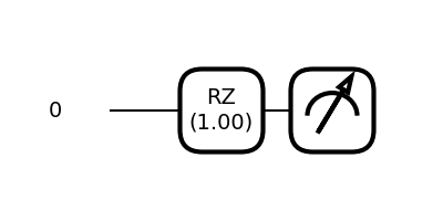
While the above may seem a little complicated, since we only use a single qubit in this tutorial, the resulting circuit is merely a single \(R_z(\theta)\) gate.

n_qubits = 1
dev = qml.device("default.qubit", wires=n_qubits, shots=None)
D_one_qubit = qml.qnode(dev)(D)
_ = qml.draw_mpl(D_one_qubit, decimals=2)(torch.tensor([1, 0]), 1, 1, True)

You may find the general function for \(D\) useful in case you want to experiment with more qubits and your own (possibly multi-dimensional) data after this tutorial.

Next, we define a circuit to calculate the probability of certain bit strings being measured in the computational basis. In our simple example, we work only with one qubit and use the default.qubit local quantum circuit simulator.

@ct.electron
@qml.qnode(dev, interface="torch", diff_method="backprop")
def get_probs(
    xt: torch.Tensor,
    t: float,
    alpha: torch.Tensor,
    gamma: torch.Tensor,
    k: int,
    U: callable,
    W: callable,
    D: callable,
    n_qubits: int,
) -> torch.Tensor:
    """Measure the probabilities for measuring each bitstring after applying a
    circuit of the form W†DWU to the |0⟩^(⊗n) state. This
    function is defined for individual sequence elements xt.
    """
    U(xt, wires=range(n_qubits))
    W(alpha, wires=range(n_qubits))
    D(gamma * t, n_qubits, k)
    qml.adjoint(W)(alpha, wires=range(n_qubits))
    return qml.probs(range(n_qubits))

To take the projector \(|0\rangle^{\otimes n} \langle 0 |^{\otimes n}\), we consider only the probability of measuring the bit string of all zeroes, which is the 0th element of the probabilities (bit strings are returned in lexicographic order).

@ct.electron
def get_callable_projector_func(
    k: int, U: callable, W: callable, D: callable, n_qubits: int, probs_func: callable
) -> callable:
    """Using get_probs() above, take only the probability of measuring the
    bitstring of all zeroes (i.e, take the projector
    |0⟩^(⊗n)⟨0|^(⊗n)) on the time devolved state.
    """
    callable_proj = lambda xt, t, alpha, gamma: probs_func(
        xt, t, alpha, gamma, k, U, W, D, n_qubits
    )[0]
    return callable_proj

We now have the necessary ingredients to build \(F(\boldsymbol{\phi}, x_t)\).

@ct.electron
def F(
    callable_proj: callable,
    xt: torch.Tensor,
    t: float,
    alpha: torch.Tensor,
    mu: torch.Tensor,
    sigma: torch.Tensor,
    gamma_length: int,
    n_samples: int,
) -> torch.Tensor:
    """Take the classical expecation value of of the projector on zero sampling
    the parameters of D from normal distributions. The expecation value is estimated
    with an average over n_samples.
    """
    # length of gamma should not exceed 2^n - 1
    gammas = sigma.abs() * torch.randn((n_samples, gamma_length)) + mu
    expectation = torch.empty(n_samples)
    for i, gamma in enumerate(gammas):
        expectation[i] = callable_proj(xt, t, alpha, gamma)
    return expectation.mean()

We now return to the matter of the penalty function \(P_{\tau}\). We choose

\[P_{\tau}(\sigma) := \frac{1}{\pi} \arctan(2 \pi \tau |\sigma|).\]

As an electron, we have

@ct.electron
def callable_arctan_penalty(tau: float) -> callable:
    """Create a callable arctan function with a single hyperparameter
    tau to penalize large entries of sigma.
    """
    prefac = 1 / (torch.pi)
    callable_pen = lambda sigma: prefac * torch.arctan(2 * torch.pi * tau * sigma.abs()).mean()
    return callable_pen

The above is a sigmoidal function chosen because it comes with the useful property of being bounded. The prefactor of \(1/\pi\) is chosen such that the final loss \(\mathcal{L}(\boldsymbol{\phi})\) is defined in the range (0, 1), as defined in the below electron.

@ct.electron
def get_loss(
    callable_proj: callable,
    batch: torch.Tensor,
    alpha: torch.Tensor,
    mu: torch.Tensor,
    sigma: torch.Tensor,
    gamma_length: int,
    n_samples: int,
    callable_penalty: callable,
) -> torch.Tensor:
    """Evaluate the loss function ℒ, defined in the background section
    for a certain set of parameters.
    """
    X_batch, T_batch = batch
    loss = torch.empty(X_batch.size()[0])
    for i in range(X_batch.size()[0]):
        # unsqueeze required for tensor to have the correct dimension for PennyLane templates
        loss[i] = (
            1
            - F(
                callable_proj,
                X_batch[i].unsqueeze(0),
                T_batch[i].unsqueeze(0),
                alpha,
                mu,
                sigma,
                gamma_length,
                n_samples,
            )
        ).square()
    return 0.5 * loss.mean() + callable_penalty(sigma)

Training the normal model

Now equipped with a loss function, we need to minimize it with a classical optimization routine. To start this optimization, however, we need some initial parameters. We can generate them with the below electron.

@ct.electron
def get_initial_parameters(
    W: callable, W_layers: int, n_qubits: int, seed: int = GLOBAL_SEED
) -> dict:
    """Randomly generate initial parameters. We need initial parameters for the
    variational circuit ansatz implementing W(alpha) and the standard deviation
    and mean (sigma and mu) for the normal distribution we sample gamma from.
    """
    torch.manual_seed(seed)
    init_alpha = torch.rand(W.shape(W_layers, n_qubits))
    init_mu = torch.rand(1)
    # Best to start sigma small and expand if needed
    init_sigma = torch.rand(1)
    init_params = {
        "alpha": (2 * torch.pi * init_alpha).clone().detach().requires_grad_(True),
        "mu": (2 * torch.pi * init_mu).clone().detach().requires_grad_(True),
        "sigma": (0.1 * init_sigma + 0.05).clone().detach().requires_grad_(True),
    }
    return init_params

Using the PyTorch interface to PennyLane, we define our final electron before running the training workflow.

@ct.electron
def train_model_gradients(
    lr: float,
    init_params: dict,
    pytorch_optimizer: callable,
    cycler: DataGetter,
    n_samples: int,
    callable_penalty: callable,
    batch_iterations: int,
    callable_proj: callable,
    gamma_length: int,
    seed=GLOBAL_SEED,
    print_intermediate=False,
) -> dict:
    """Train the QVR model (minimize the loss function) with respect to the
    variational parameters using gradient-based training. You need to pass a
    PyTorch optimizer and a learning rate (lr).
    """
    torch.manual_seed(seed)
    opt = pytorch_optimizer(init_params.values(), lr=lr)
    alpha = init_params["alpha"]
    mu = init_params["mu"]
    sigma = init_params["sigma"]

    def closure():
        opt.zero_grad()
        loss = get_loss(
            callable_proj, next(cycler), alpha, mu, sigma, gamma_length, n_samples, callable_penalty
        )
        loss.backward()
        return loss

    loss_history = []
    for i in range(batch_iterations):
        loss = opt.step(closure)
        loss_history.append(loss.item())
        if batch_iterations % 10 == 0 and print_intermediate:
            print(f"Iteration number {i}\n Current loss {loss.item()}\n")

    results_dict = {
        "opt_params": {
            "alpha": opt.param_groups[0]["params"][0],
            "mu": opt.param_groups[0]["params"][1],
            "sigma": opt.param_groups[0]["params"][2],
        },
        "loss_history": loss_history,
    }
    return results_dict

Now, enter our first @ct.lattice. This combines the above electrons, eventually returning the optimal parameters \(\boldsymbol{\phi}^{\star}\) and the loss with batch iterations.

@ct.lattice
def training_workflow(
    U: callable,
    W: callable,
    D: callable,
    n_qubits: int,
    k: int,
    probs_func: callable,
    W_layers: int,
    gamma_length: int,
    n_samples: int,
    p: int,
    num_series: int,
    noise_amp: float,
    t_init: float,
    t_end: float,
    batch_size: int,
    tau: float,
    pytorch_optimizer: callable,
    lr: float,
    batch_iterations: int,
):
    """
    Combine all of the previously defined electrons to do an entire training workflow,
    including (1) generating synthetic data, (2) packaging it into training cyclers
    (3) preparing the quantum functions and (4) optimizing the loss function with
    gradient based optimization. You can find definitions for all of the arguments
    by looking at the electrons and text cells above.
    """

    X, T = generate_normal_time_series_set(p, num_series, noise_amp, t_init, t_end)
    Xtr = make_atomized_training_set(X, T)
    cycler = get_training_cycler(Xtr, batch_size)
    init_params = get_initial_parameters(W, W_layers, n_qubits)
    callable_penalty = callable_arctan_penalty(tau)
    callable_proj = get_callable_projector_func(k, U, W, D, n_qubits, probs_func)
    results_dict = train_model_gradients(
        lr,
        init_params,
        pytorch_optimizer,
        cycler,
        n_samples,
        callable_penalty,
        batch_iterations,
        callable_proj,
        gamma_length,
        print_intermediate=False,
    )
    return results_dict

Before running this workflow, we define all of the input parameters.

general_options = {
    "U": qml.AngleEmbedding,
    "W": qml.StronglyEntanglingLayers,
    "D": D,
    "n_qubits": 1,
    "probs_func": get_probs,
    "gamma_length": 1,
    "n_samples": 10,
    "p": 25,
    "num_series": 25,
    "noise_amp": 0.1,
    "t_init": 0.1,
    "t_end": 2 * torch.pi,
    "k": 1,
}

training_options = {
    "batch_size": 10,
    "tau": 5,
    "pytorch_optimizer": torch.optim.Adam,
    "lr": 0.01,
    "batch_iterations": 100,
    "W_layers": 2,
}

training_options.update(general_options)

We can now dispatch the lattice to the Covalent server.

tr_dispatch_id = ct.dispatch(training_workflow)(**training_options)

If you are running the notebook version of this tutorial, if you navigate to http://localhost:48008/ you can view the workflow on the Covalent GUI. It will look like the screenshot below, showing nicely how all of the electrons defined above interact with each other in the workflow. You can also track the progress of the calculation here.

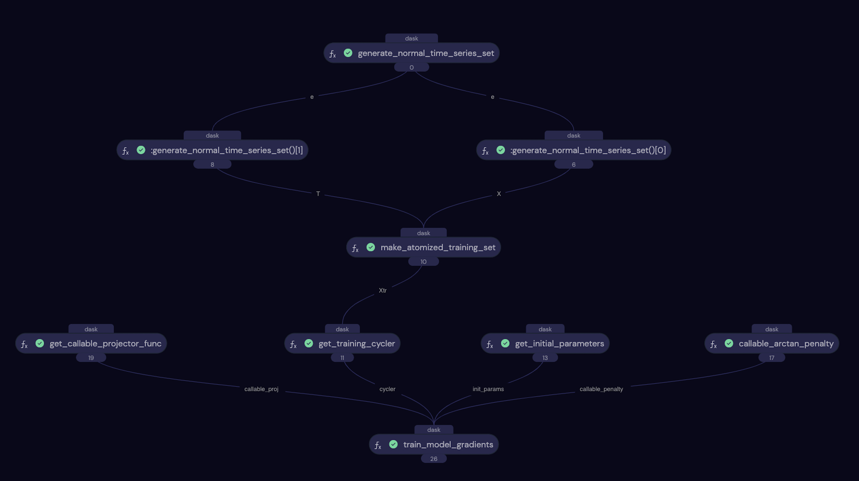
A screenshot of the Covalent GUI for the training workflow.

We now pull the results back from the Covalent server:

ct_tr_results = ct.get_result(dispatch_id=tr_dispatch_id, wait=True)
results_dict = ct_tr_results.result

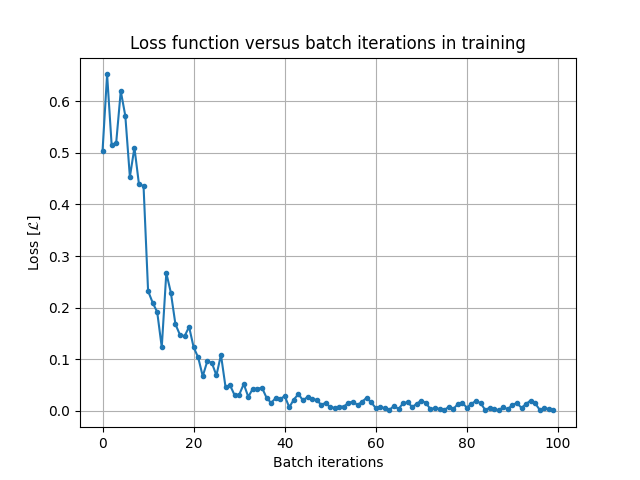
and take a look at the training loss history:

plt.figure()
plt.plot(results_dict["loss_history"], ".-")
plt.ylabel("Loss [$\mathcal{L}$]")
plt.xlabel("Batch iterations")
plt.title("Loss function versus batch iterations in training")
plt.grid()

Tuning the threshold \(\zeta\)

When we have access to labelled anomalous series (as we do in our toy problem here, often not the case in reality), we can tune the threshold \(\zeta\) to maximize some success metric. We choose to maximize the accuracy score as defined using the three electrons below.

@ct.electron
def get_preds_given_threshold(zeta: float, scores: torch.Tensor) -> torch.Tensor:
    """For a given threshold, get the predicted labels (1 or -1), given the anomaly scores."""
    return torch.tensor([-1 if score > zeta else 1 for score in scores])


@ct.electron
def get_truth_labels(
    normal_series_set: torch.Tensor, anomalous_series_set: torch.Tensor
) -> torch.Tensor:
    """Get a 1D tensor containing the truth values (1 or -1) for a given set of
    time series.
    """
    norm = torch.ones(normal_series_set.size()[0])
    anom = -torch.ones(anomalous_series_set.size()[0])
    return torch.cat([norm, anom])


@ct.electron
def get_accuracy_score(pred: torch.Tensor, truth: torch.Tensor) -> torch.Tensor:
    """Given the predictions and truth values, return a number between 0 and 1
    indicating the accuracy of predictions.
    """
    return torch.sum(pred == truth) / truth.size()[0]

Then, knowing the anomaly scores \(a_X(y)\) for a validation data set, we can scan through various values of \(\zeta\) on a fine 1D grid and calcuate the accuracy score. Our goal is to pick the \(\zeta\) with the largest accuracy score.

@ct.electron
def threshold_scan_acc_score(
    scores: torch.Tensor, truth_labels: torch.Tensor, zeta_min: float, zeta_max: float, steps: int
) -> torch.Tensor:
    """Given the anomaly scores and truth values,
    scan over a range of thresholds = [zeta_min, zeta_max] with a
    fixed number of steps, calculating the accuracy score at each point.
    """
    accs = torch.empty(steps)
    for i, zeta in enumerate(torch.linspace(zeta_min, zeta_max, steps)):
        preds = get_preds_given_threshold(zeta, scores)
        accs[i] = get_accuracy_score(preds, truth_labels)
    return accs


@ct.electron
def get_anomaly_score(
    callable_proj: callable,
    y: torch.Tensor,
    T: torch.Tensor,
    alpha_star: torch.Tensor,
    mu_star: torch.Tensor,
    sigma_star: torch.Tensor,
    gamma_length: int,
    n_samples: int,
    get_time_resolved: bool = False,
):
    """Get the anomaly score for an input time series y. We need to pass the
    optimal parameters (arguments with suffix _star). Optionally return the
    time-resolved score (the anomaly score contribution at a given t).
    """
    scores = torch.empty(T.size()[0])
    for i in range(T.size()[0]):
        scores[i] = (
            1
            - F(
                callable_proj,
                y[i].unsqueeze(0),
                T[i].unsqueeze(0),
                alpha_star,
                mu_star,
                sigma_star,
                gamma_length,
                n_samples,
            )
        ).square()
    if get_time_resolved:
        return scores, scores.mean()
    else:
        return scores.mean()


@ct.electron
def get_norm_and_anom_scores(
    X_norm: torch.Tensor,
    X_anom: torch.Tensor,
    T: torch.Tensor,
    callable_proj: callable,
    model_params: dict,
    gamma_length: int,
    n_samples: int,
) -> torch.Tensor:
    """Get the anomaly scores assigned to input normal and anomalous time series instances.
    model_params is a dictionary containing the optimal model parameters.
    """
    alpha = model_params["alpha"]
    mu = model_params["mu"]
    sigma = model_params["sigma"]
    norm_scores = torch.tensor(
        [
            get_anomaly_score(callable_proj, xt, T, alpha, mu, sigma, gamma_length, n_samples)
            for xt in X_norm
        ]
    )
    anom_scores = torch.tensor(
        [
            get_anomaly_score(callable_proj, xt, T, alpha, mu, sigma, gamma_length, n_samples)
            for xt in X_anom
        ]
    )
    return torch.cat([norm_scores, anom_scores])

We now create our second @ct.lattice. We are to test the optimal model against two random models. If our model is trainable, we should see that the trained model is better.

@ct.lattice
def threshold_tuning_workflow(
    opt_params: dict,
    gamma_length: int,
    n_samples: int,
    probs_func: callable,
    zeta_min: float,
    zeta_max: float,
    steps: int,
    p: int,
    num_series: int,
    noise_amp: float,
    spike_amp: float,
    max_duration: int,
    t_init: float,
    t_end: float,
    k: int,
    U: callable,
    W: callable,
    D: callable,
    n_qubits: int,
    random_model_seeds: torch.Tensor,
    W_layers: int,
) -> tuple:
    """A workflow for tuning the threshold value zeta, in order to maximize the accuracy score
    for a validation data set. Results are tested against random models at their optimal zetas.
    """
    # Generate datasets
    X_val_norm, T = generate_normal_time_series_set(p, num_series, noise_amp, t_init, t_end)
    X_val_anom, T = generate_anomalous_time_series_set(
        p, num_series, noise_amp, spike_amp, max_duration, t_init, t_end
    )
    truth_labels = get_truth_labels(X_val_norm, X_val_anom)

    # Initialize quantum functions
    callable_proj = get_callable_projector_func(k, U, W, D, n_qubits, probs_func)

    accs_list = []
    scores_list = []
    # Evaluate optimal model
    scores = get_norm_and_anom_scores(
        X_val_norm, X_val_anom, T, callable_proj, opt_params, gamma_length, n_samples
    )
    accs_opt = threshold_scan_acc_score(scores, truth_labels, zeta_min, zeta_max, steps)
    accs_list.append(accs_opt)
    scores_list.append(scores)

    # Evaluate random models
    for seed in random_model_seeds:
        rand_params = get_initial_parameters(W, W_layers, n_qubits, seed)
        scores = get_norm_and_anom_scores(
            X_val_norm, X_val_anom, T, callable_proj, rand_params, gamma_length, n_samples
        )
        accs_list.append(threshold_scan_acc_score(scores, truth_labels, zeta_min, zeta_max, steps))
        scores_list.append(scores)
    return accs_list, scores_list

We now set the input parameters.

threshold_tuning_options = {
    "spike_amp": 0.4,
    "max_duration": 5,
    "zeta_min": 0,
    "zeta_max": 1,
    "steps": 100000,
    "random_model_seeds": [0, 1],
    "W_layers": 2,
    "opt_params": results_dict["opt_params"],
}

threshold_tuning_options.update(general_options)

As before, we dispatch the lattice to the Covalent server.

val_dispatch_id = ct.dispatch(threshold_tuning_workflow)(**threshold_tuning_options)
ct_val_results = ct.get_result(dispatch_id=val_dispatch_id, wait=True)
accs_list, scores_list = ct_val_results.result

Now, we can plot the results:

zeta_xlims = [(0, 0.001), (0.25, 0.38), (0.25, 0.38)]
titles = ["Trained model", "Random model 1", "Random model 2"]
zetas = torch.linspace(
    threshold_tuning_options["zeta_min"],
    threshold_tuning_options["zeta_max"],
    threshold_tuning_options["steps"],
)
fig, axs = plt.subplots(ncols=3, nrows=2, sharey="row")
for i in range(3):
    axs[0, i].plot(zetas, accs_list[i])
    axs[0, i].set_xlim(zeta_xlims[i])
    axs[0, i].set_xlabel("Threshold [$\zeta$]")
    axs[0, i].set_title(titles[i])
    axs[1, i].boxplot(
        [
            scores_list[i][0 : general_options["num_series"]],
            scores_list[i][general_options["num_series"] : -1],
        ],
        labels=["Normal", "Anomalous"],
    )
    axs[1, i].set_yscale("log")
    axs[1, i].axhline(
        zetas[torch.argmax(accs_list[i])], color="k", linestyle=":", label="Optimal $\zeta$"
    )
    axs[1, i].legend()
axs[0, 0].set_ylabel("Accuracy score")
axs[1, 0].set_ylabel("Anomaly score [$a_X(y)$]")
fig.tight_layout()

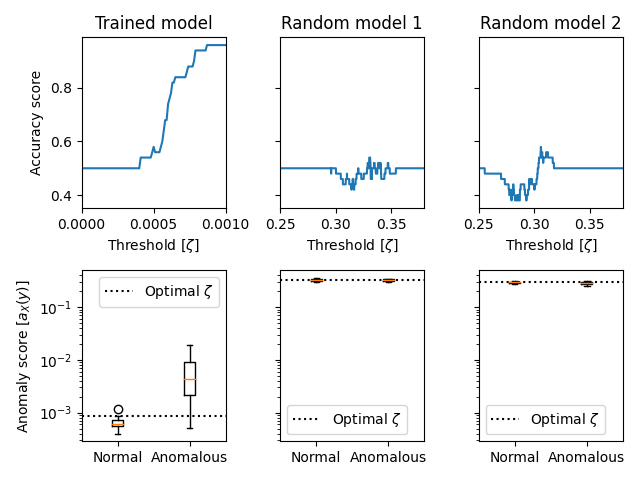
Parsing the above, we can see that the optimal model achieves high accuracy when the threshold is tuned using the validation data. On the other hand, the random models return mostly random results (sometimes even worse than random guesses), regardless of how we set the threshold.

Testing the model

Now with optimal thresholds for our optimized and random models, we can perform testing. We already have all of the electrons to do this, so we create the @ct.lattice

@ct.lattice
def testing_workflow(
    opt_params: dict,
    gamma_length: int,
    n_samples: int,
    probs_func: callable,
    best_zetas: list,
    p: int,
    num_series: int,
    noise_amp: float,
    spike_amp: float,
    max_duration: int,
    t_init: float,
    t_end: float,
    k: int,
    U: callable,
    W: callable,
    D: callable,
    n_qubits: int,
    random_model_seeds: torch.Tensor,
    W_layers: int,
) -> list:
    """A workflow for calculating anomaly scores for a set of testing time series
    given an optimal model and set of random models. We use the optimal zetas found in threshold tuning.
    """
    # Generate time series
    X_val_norm, T = generate_normal_time_series_set(p, num_series, noise_amp, t_init, t_end)
    X_val_anom, T = generate_anomalous_time_series_set(
        p, num_series, noise_amp, spike_amp, max_duration, t_init, t_end
    )
    truth_labels = get_truth_labels(X_val_norm, X_val_anom)

    # Prepare quantum functions
    callable_proj = get_callable_projector_func(k, U, W, D, n_qubits, probs_func)

    accs_list = []
    # Evaluate optimal model
    scores = get_norm_and_anom_scores(
        X_val_norm, X_val_anom, T, callable_proj, opt_params, gamma_length, n_samples
    )
    preds = get_preds_given_threshold(best_zetas[0], scores)
    accs_list.append(get_accuracy_score(preds, truth_labels))
    # Evaluate random models
    for zeta, seed in zip(best_zetas[1:], random_model_seeds):
        rand_params = get_initial_parameters(W, W_layers, n_qubits, seed)
        scores = get_norm_and_anom_scores(
            X_val_norm, X_val_anom, T, callable_proj, rand_params, gamma_length, n_samples
        )
        preds = get_preds_given_threshold(zeta, scores)
        accs_list.append(get_accuracy_score(preds, truth_labels))
    return accs_list

We dispatch it to the Covalent server with the appropriate parameters.

testing_options = {
    "spike_amp": 0.4,
    "max_duration": 5,
    "best_zetas": [zetas[torch.argmax(accs)] for accs in accs_list],
    "random_model_seeds": [0, 1],
    "W_layers": 2,
    "opt_params": results_dict["opt_params"],
}

testing_options.update(general_options)

test_dispatch_id = ct.dispatch(testing_workflow)(**testing_options)
ct_test_results = ct.get_result(dispatch_id=test_dispatch_id, wait=True)
accs_list = ct_test_results.result

Finally, we plot the results below.

plt.figure()
plt.bar([1, 2, 3], accs_list)
plt.axhline(0.5, color="k", linestyle=":", label="Random accuracy")
plt.xticks([1, 2, 3], ["Trained model", "Random model 1", "Random model 2"])
plt.ylabel("Accuracy score")
plt.title("Accuracy scores for trained and random models")
leg = plt.legend()

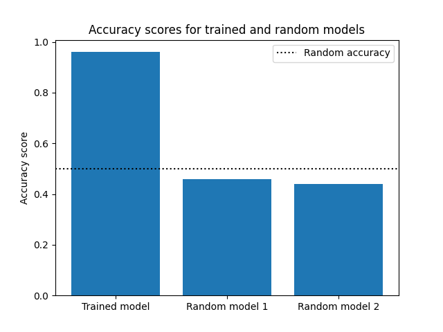
As can be seen, once more, the trained model is far more accurate than the random models. Awesome! Now that we’re done with the calculations in this tutorial, we just need to remember to shut down the Covalent server

# Shut down the covalent server
stop = os.system("covalent stop")

Conclusions

We’ve now reached the end of this tutorial! Quickly recounting what we have learnt, we:

1. Learnt the background of how to detect anomalous time series instances, quantumly,

2. Learnt how to build the code to achieve this using PennyLane and PyTorch, and,

3. Learnt the basics of Covalent: a workflow orchestration tool for heterogeneous computation

If you want to learn more about QVR, you should consult the paper 1 where we generalize the math a little and test the algorithm on less trivial time series data than was dealt with in this tutorial. We also ran some experiments on real quantum computers, enhancing our results using error mitigation techniques. If you want to play some more with Covalent, check us out on GitHub and/or engage with other tutorials in our documentation.

References

1(1,2,3,4)

Baker, Jack S. et al. “Quantum Variational Rewinding for Time Series Anomaly Detection.” arXiv preprint arXiv:2210.164388 (2022).

2

Stone, Marshall H. “On one-parameter unitary groups in Hilbert space.” Annals of Mathematics, 643-648, doi:10.2307/1968538 (1932).

3

Welch, Jonathan et al. “Efficient quantum circuits for diagonal unitaries without ancillas”, New Journal of Physics, 16, 033040 doi:10.1088/1367-2630/16/3/033040 (2014).

4

Cîrstoiu, Cristina et al. “Variational fast forwarding for quantum simulation beyond the coherence time”, npj Quantum Information, 6, doi:10.1038/s41534-020-00302-0, (2020)

About the authors

Jack S. Baker

Jack is a quantum algorithms researcher at Agnostiq specializing in quantum machine learning and optimization.

Santosh Kumar Radha

Santosh is the head of research and development and product lead at Agnostiq.

demos/tutorial_univariate_qvr

 

Download Python script

 

Download Notebook

 

View on GitHub