Parameter-shift rules

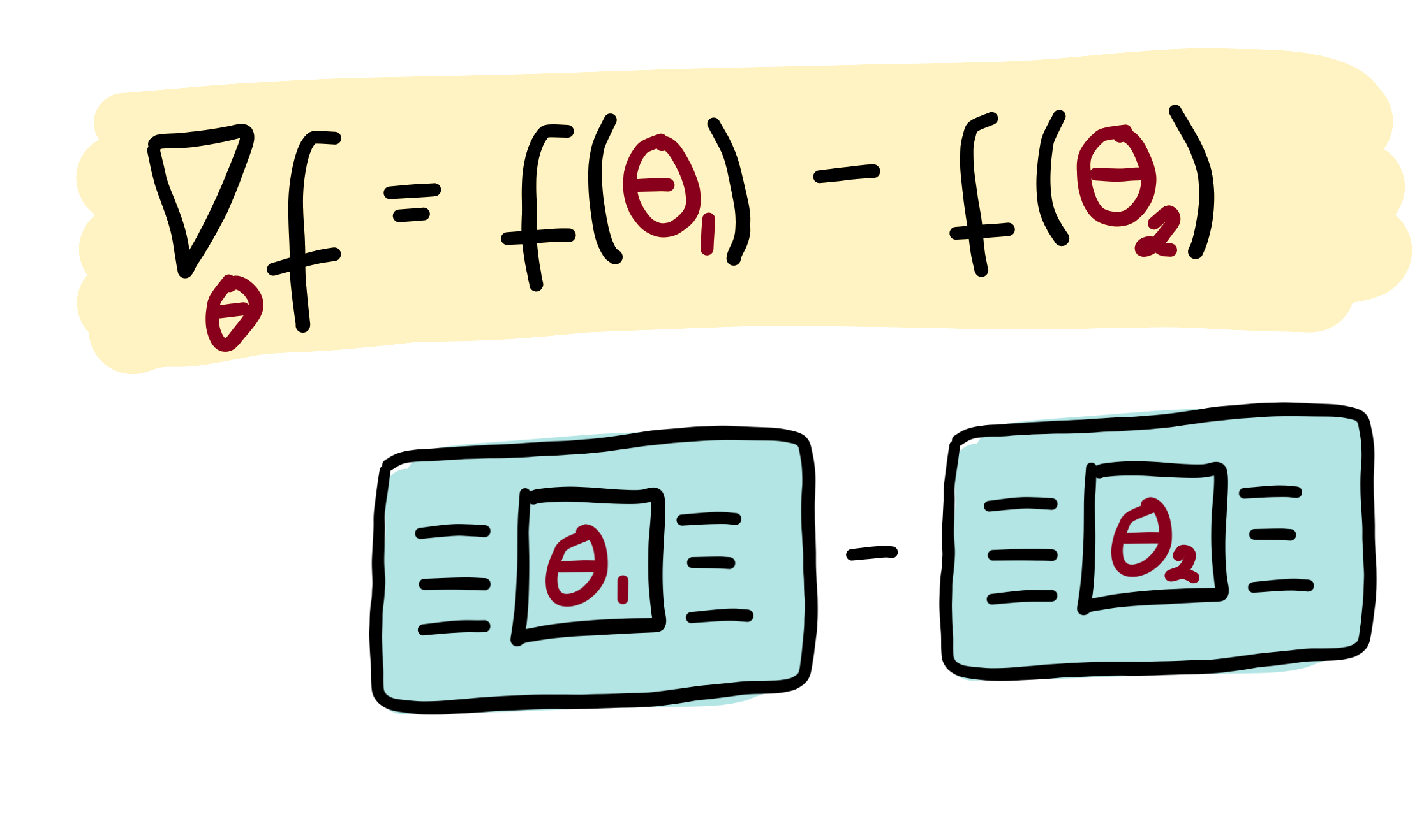
The output of a variational circuit (i.e., the expectation of an observable) can be written as a “quantum function” \(f(\theta)\) parametrized by \(\theta = \theta_1, \theta_2, \dots\). The partial derivative of \(f(\theta)\) can in many cases be expressed as a linear combination of other quantum functions. Importantly, these other quantum functions typically use the same circuit, differing only in a shift of the argument. This means that partial derivatives of a variational circuit can be computed by using the same variational circuit architecture.

Recipes of how to get partial derivatives by evaluated parameter-shifted instances of a variational circuit are called parameter-shift rules, and have been first introduced to quantum machine learning in Mitarai et al. (2018), and extended in Schuld et al. (2018).

Making a rough analogy to classically computable functions, this is similar to how the derivative of the function \(f(x)=\sin(x)\) is identical to \(\frac{1}{2}\sin(x+\frac{\pi}{2}) - \frac{1}{2}\sin(x-\frac{\pi}{2})\). So the same underlying algorithm can be reused to compute both \(\sin(x)\) and its derivative (by evaluating at \(x\pm\frac{\pi}{2}\)). This intuition holds for many quantum functions of interest: the same circuit can be used to compute both the quantum function and the gradient of the quantum function 1.

A more technical explanation

Quantum circuits are specified by a sequence of gates. The unitary transformation carried out by the circuit can thus be broken down into a product of unitaries:

\[U(x; \theta) = U_N(\theta_{N}) U_{N-1}(\theta_{N-1}) \cdots U_i(\theta_i) \cdots U_1(\theta_1) U_0(x).\]

Each of these gates is unitary, and therefore must have the form \(U_{j}(\gamma_j)=\exp{(i\gamma_j H_j)}\) where \(H_j\) is a Hermitian operator which generates the gate and \(\gamma_j\) is the gate parameter. We have omitted which wire each unitary acts on, since it is not necessary for the following discussion.

Note

In this example, we have used the input \(x\) as the argument for gate \(U_0\) and the parameters \(\theta\) for the remaining gates. This is not required. Inputs and parameters can be arbitrarily assigned to different gates.

A single parameterized gate

Let us single out a single parameter \(\theta_i\) and its associated gate \(U_i(\theta_i)\). For simplicity, we remove all gates except \(U_i(\theta_i)\) and \(U_0(x)\) for the moment. In this case, we have a simplified quantum circuit function

\[f(x; \theta_i) = \langle 0 | U_0^\dagger(x)U_i^\dagger(\theta_i)\hat{B}U_i(\theta_i)U_0(x) | 0 \rangle = \langle x | U_i^\dagger(\theta_i)\hat{B}U_i(\theta_i) | x \rangle.\]

For convenience, we rewrite the unitary conjugation as a linear transformation \(\mathcal{M}_{\theta_i}\) acting on the operator \(\hat{B}\):

\[U_i^\dagger(\theta_i)\hat{B}U_i(\theta_i) = \mathcal{M}_{\theta_i}(\hat{B}).\]

The transformation \(\mathcal{M}_{\theta_i}\) depends smoothly on the parameter \(\theta_i\), so this quantum function will have a well-defined gradient:

\[\nabla_{\theta_i}f(x; \theta_i) = \langle x | \nabla_{\theta_i}\mathcal{M}_{\theta_i}(\hat{B}) | x \rangle \in \mathbb{R}.\]

The key insight is that we can, in many cases of interest, express this gradient as a linear combination of the same transformation \(\mathcal{M}\), but with different parameters. Namely,

\[\nabla_{\theta_i}\mathcal{M}_{\theta_i}(\hat{B}) = c[\mathcal{M}_{\theta_i + s}(\hat{B}) - \mathcal{M}_{\theta_i - s}(\hat{B})],\]

where the multiplier \(c\) and the shift \(s\) are determined completely by the type of transformation \(\mathcal{M}\) and independent of the value of \(\theta_i\).

Note

While this construction bears some resemblance to the numerical finite-difference method for computing derivatives, here \(s\) is finite rather than infinitesimal.

Multiple parameterized gates

To complete the story, we now go back to the case where there are many gates in the circuit. We can absorb any gates applied before gate \(i\) into the initial state: \(|\psi_{i-1}\rangle = U_{i-1}(\theta_{i-1}) \cdots U_{1}(\theta_{1})U_{0}(x)|0\rangle\). Similarly, any gates applied after gate \(i\) are combined with the observable \(\hat{B}\): \(\hat{B}_{i+1} = U_{N}^\dagger(\theta_{N}) \cdots U_{i+1}^\dagger(\theta_{i+1}) \hat{B} U_{i+1}(\theta_{i+1}) \cdots U_{N}(\theta_{N})\).

With this simplification, the quantum circuit function becomes

\[f(x; \theta) = \langle \psi_{i-1} | U_i^\dagger(\theta_i) \hat{B}_{i+1} U_i(\theta_i) | \psi_{i-1} \rangle = \langle \psi_{i-1} | \mathcal{M}_{\theta_i} (\hat{B}_{i+1}) | \psi_{i-1} \rangle,\]

and its gradient is

\[\nabla_{\theta_i}f(x; \theta) = \langle \psi_{i-1} | \nabla_{\theta_i}\mathcal{M}_{\theta_i} (\hat{B}_{i+1}) | \psi_{i-1} \rangle.\]

This gradient has the exact same form as the single-gate case, except we modify the state \(|x\rangle \rightarrow |\psi_{i-1}\rangle\) and the measurement operator \(\hat{B}\rightarrow\hat{B}_{i+1}\). In terms of the circuit, this means we can leave all other gates as they are, and only modify gate \(U(\theta_i)\) when we want to differentiate with respect to the parameter \(\theta_i\).

Note

Sometimes we may want to use the same classical parameter with multiple gates in the circuit. Due to the product rule, the total gradient will then involve contributions from each gate that uses that parameter.

Pauli gate example

Consider a quantum computer with parameterized gates of the form

\[U_i(\theta_i)=\exp\left(-i\tfrac{\theta_i}{2}\hat{P}_i\right),\]

where \(\hat{P}_i=\hat{P}_i^\dagger\) is a Pauli operator.

The gradient of this unitary is

\[\nabla_{\theta_i}U_i(\theta_i) = -\tfrac{i}{2}\hat{P}_i U_i(\theta_i) = -\tfrac{i}{2}U_i(\theta_i)\hat{P}_i .\]

Substituting this into the quantum circuit function \(f(x; \theta)\), we get

\begin{align} \nabla_{\theta_i}f(x; \theta) = & \frac{i}{2}\langle \psi_{i-1} | U_i^\dagger(\theta_i) \left( P_i \hat{B}_{i+1} - \hat{B}_{i+1} P_i \right) U_i(\theta_i)| \psi_{i-1} \rangle \\ = & \frac{i}{2}\langle \psi_{i-1} | U_i^\dagger(\theta_i) \left[P_i, \hat{B}_{i+1}\right]U_i(\theta_i) | \psi_{i-1} \rangle, \end{align}

where \([X,Y]=XY-YX\) is the commutator.

We now make use of the following mathematical identity for commutators involving Pauli operators (Mitarai et al. (2018)):

\[\left[ \hat{P}_i, \hat{B} \right] = -i\left(U_i^\dagger\left(\tfrac{\pi}{2}\right)\hat{B}U_i\left(\tfrac{\pi}{2}\right) - U_i^\dagger\left(-\tfrac{\pi}{2}\right)\hat{B}U_i\left(-\tfrac{\pi}{2}\right) \right).\]

Substituting this into the previous equation, we obtain the gradient expression

\begin{align} \nabla_{\theta_i}f(x; \theta) = & \hphantom{-} \tfrac{1}{2} \langle \psi_{i-1} | U_i^\dagger\left(\theta_i + \tfrac{\pi}{2} \right) \hat{B}_{i+1} U_i\left(\theta_i + \tfrac{\pi}{2} \right) | \psi_{i-1} \rangle \\ & - \tfrac{1}{2} \langle \psi_{i-1} | U_i^\dagger\left(\theta_i - \tfrac{\pi}{2} \right) \hat{B}_{i+1} U_i\left(\theta_i - \tfrac{\pi}{2} \right) | \psi_{i-1} \rangle. \end{align}

Finally, we can rewrite this in terms of quantum functions:

\[\nabla_{\theta}f(x; \theta) = \tfrac{1}{2}\left[ f(x; \theta + \tfrac{\pi}{2}) - f(x; \theta - \tfrac{\pi}{2}) \right].\]

Gaussian gate example

For quantum devices with continuous-valued operators, such as photonic quantum computers, it is convenient to employ the Heisenberg picture, i.e., to track how the gates \(U_i(\theta_i)\) transform the final measurement operator \(\hat{B}\).

As an example, we consider the Squeezing gate. In the Heisenberg picture, the Squeezing gate causes the quadrature operators \(\hat{x}\) and \(\hat{p}\) to become rescaled:

\begin{align} \mathcal{M}^S_r(\hat{x}) = & S^\dagger(r)\hat{x}S(r) \\ = & e^{-r}\hat{x} \end{align}

and

\begin{align} \mathcal{M}^S_r(\hat{p}) = & S^\dagger(r)\hat{p}S(r) \\ = & e^{r}\hat{p}. \end{align}

Expressing this in matrix notation, we have

\begin{align} \begin{bmatrix} \hat{x} \\ \hat{p} \end{bmatrix} \rightarrow \begin{bmatrix} e^{-r} & 0 \\ 0 & e^r \end{bmatrix} \begin{bmatrix} \hat{x} \\ \hat{p} \end{bmatrix}. \end{align}

The gradient of this transformation can easily be found:

\begin{align} \nabla_r \begin{bmatrix} e^{-r} & 0 \\ 0 & e^r \end{bmatrix} = \begin{bmatrix} -e^{-r} & 0 \\ 0 & e^r \end{bmatrix}. \end{align}

We notice that this can be rewritten this as a linear combination of squeeze operations:

\begin{align} \begin{bmatrix} -e^{-r} & 0 \\ 0 & e^r \end{bmatrix} = \frac{1}{2\sinh(s)} \left( \begin{bmatrix} e^{-(r+s)} & 0 \\ 0 & e^{r+s} \end{bmatrix} - \begin{bmatrix} e^{-(r-s)} & 0 \\ 0 & e^{r-s} \end{bmatrix} \right), \end{align}

where \(s\) is an arbitrary nonzero shift 2.

As before, assume that an input \(y\) has already been embedded into a quantum state \(|y\rangle = U_0(y)|0\rangle\) before we apply the squeeze gate. If we measure the \(\hat{x}\) operator, we will have the following quantum circuit function:

\[f(y;r) = \langle y | \mathcal{M}^S_r (\hat{x}) | y \rangle.\]

Finally, its gradient can be expressed as

\begin{align} \nabla_r f(y;r) = & \frac{1}{2\sinh(s)} \left[ \langle y | \mathcal{M}^S_{r+s} (\hat{x}) | y \rangle -\langle y | \mathcal{M}^S_{r-s} (\hat{x}) | y \rangle \right] \\ = & \frac{1}{2\sinh(s)}\left[f(y; r+s) - f(y; r-s)\right]. \end{align}

Note

For simplicity of the discussion, we have set the phase angle of the Squeezing gate to be zero. In the general case, Squeezing is a two-parameter gate, containing a squeezing magnitude and a squeezing angle. However, we can always decompose the two-parameter form into a Squeezing gate like the one above, followed by a Rotation gate.

Footnotes

1

This should be contrasted with software which can perform automatic differentiation on classical simulations of quantum circuits, such as Strawberry Fields.

2

In situations where no formula for automatic quantum gradients is known, one can fall back to approximate gradient estimation using numerical methods.

3

In physical experiments, it is beneficial to choose \(s\) so that the additional squeezing is small. However, there is a tradeoff, because we also want to make sure \(\frac{1}{2\sinh(s)}\) does not blow up numerically.

glossary/parameter_shift

 

Download Python script

 

Download Notebook

 

View on GitHub