Note
Click here to download the full example code
Optimizing a quantum optical neural network
Author: Theodor Isacsson — Posted: 05 August 2020. Last updated: 08 March 2022.
Warning
This demo is only compatible with PennyLane version 0.29 or below.
This tutorial is based on a paper from Steinbrecher et al. (2019) which explores a Quantum Optical Neural Network (QONN) based on Fock states. Similar to the continuous-variable quantum neural network (CV QNN) model described by Killoran et al. (2018), the QONN attempts to apply neural networks and deep learning theory to the quantum case, using quantum data as well as a quantum hardware-based architecture.
We will focus on constructing a QONN as described in Steinbrecher et al. and training it to work as a basic CNOT gate using a “dual-rail” state encoding. This tutorial also provides a working example of how to use third-party optimization libraries with PennyLane; in this case, NLopt will be used.
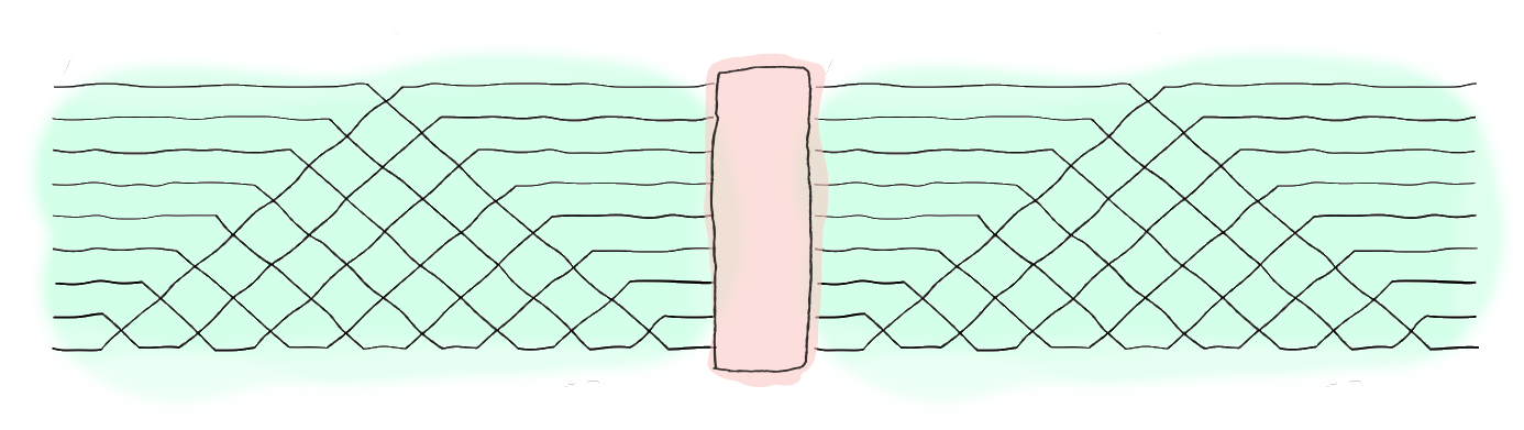
A quantum optical neural network using the Reck encoding (green) with a Kerr non-linear layer (red)
Background
The QONN is an optical architecture consisting of layers of linear unitaries, using the encoding described in Reck et al. (1994), and Kerr non-linearities applied on all involved optical modes. This setup can be constructed using arrays of beamsplitters and programmable phase shifts along with some form of Kerr non-linear material.
By constructing a cost function based on the input-output relationship of the QONN, using the programmable phase-shift variables as optimization parameters, it can be trained to both act as an arbitrary quantum gate or to be able to generalize on previously unseen data. This is very similar to classical neural networks, and many classical machine learning task can in fact also be solved by these types of quantum deep neural networks.
Code and simulations
The first thing we need to do is to import PennyLane, NumPy, as well as an optimizer. Here we use a wrapped version of NumPy supplied by PennyLane which uses Autograd to wrap essential functions to support automatic differentiation.
There are many optimizers to choose from. We could either use an
optimizer from the pennylane.optimize module or we could use a
third-party optimizer. In this case we will use the Nlopt library
which has several fast implementations of both gradient-free and
gradient-based optimizers.
import pennylane as qml
from pennylane import numpy as np

import nlopt
We create a Strawberry Fields simulator device with as many quantum modes (or wires) as we want our quantum-optical neural network to have. Four modes are used for this demonstration, due to the use of a dual-rail encoding. The cutoff dimension is set to the same value as the number of wires (a lower cutoff value will cause loss of information, while a higher value might use unnecessary resources without any improvement).
dev = qml.device("strawberryfields.fock", wires=4, cutoff_dim=4)
Note
You will need to have Strawberry Fields as well as the Strawberry Fields plugin for PennyLane installed for this tutorial to work.
Creating the QONN
Create a layer function which defines one layer of the QONN, consisting of a linear interferometer (i.e., an array of beamsplitters and phase shifts) and a non-linear Kerr interaction layer. Both the interferometer and the non-linear layer are applied to all modes. The triangular mesh scheme, described in Reck et al. (1994) is chosen here due to its use in the paper from Steinbrecher et al., although any other interferometer scheme should work equally well. Some might even be slightly faster than the one we use here.
def layer(theta, phi, wires):
    M = len(wires)
    phi_nonlinear = np.pi / 2

    qml.Interferometer(
        theta, phi, np.zeros(M), wires=wires, mesh="triangular",
    )

    for i in wires:
        qml.Kerr(phi_nonlinear, wires=i)
Next, we define the full QONN by building each layer one-by-one and then
measuring the mean photon number of each mode. The parameters to be
optimized are all contained in var, where each element in var is
a list of parameters theta and phi for a specific layer.
@qml.qnode(dev)
def quantum_neural_net(var, x):
    wires = list(range(len(x)))

    # Encode input x into a sequence of quantum fock states
    for i in wires:
        qml.FockState(x[i], wires=i)

    # "layer" subcircuits
    for i, v in enumerate(var):
        layer(v[: len(v) // 2], v[len(v) // 2 :], wires)

    return [qml.expval(qml.NumberOperator(w)) for w in wires]
Defining the cost function
A helper function is needed to calculate the normalized square loss of
two vectors. The square loss function returns a value between 0 and 1,
where 0 means that labels and predictions are equal and 1 means
that the vectors are fully orthogonal.
def square_loss(labels, predictions):
    term = 0
    for l, p in zip(labels, predictions):
        lnorm = l / np.linalg.norm(l)
        pnorm = p / np.linalg.norm(p)

        term = term + np.abs(np.dot(lnorm, pnorm.T)) ** 2

    return 1 - term / len(labels)
Finally, we define the cost function to be used during optimization. It
collects the outputs from the QONN (predictions) for each input
(data_inputs) and then calculates the square loss between the
predictions and the true outputs (labels).
def cost(var, data_input, labels):
    predictions = np.array([quantum_neural_net(var, x) for x in data_input])
    sl = square_loss(labels, predictions)

    return sl
Optimizing for the CNOT gate
For this tutorial we will train the network to function as a CNOT gate. That is, it should transform the input states in the following way:

We need to choose the inputs X and the corresponding labels Y. They are
defined using the dual-rail encoding, meaning that \(|0\rangle = [1, 0]\)
(as a vector in the Fock basis of a single mode), and
\(|1\rangle = [0, 1]\). So a CNOT transformation of \(|1\rangle|0\rangle = |10\rangle = [0, 1, 1, 0]\)
would give \(|11\rangle = [0, 1, 0, 1]\).
Furthermore, we want to make sure that the gradient isn’t calculated with regards to the inputs or the labels. We can do this by marking them with requires_grad=False.
# Define the CNOT input-output states (dual-rail encoding) and initialize
# them as non-differentiable.

X = np.array([[1, 0, 1, 0],
              [1, 0, 0, 1],
              [0, 1, 1, 0],
              [0, 1, 0, 1]], requires_grad=False)

Y = np.array([[1, 0, 1, 0],
              [1, 0, 0, 1],
              [0, 1, 0, 1],
              [0, 1, 1, 0]], requires_grad=False)
At this stage we could play around with other input-output combinations; just keep in mind that the input states should contain the same total number of photons as the output, since we want to use the dual-rail encoding. Also, since the QONN will act upon the states as a unitary operator, there must be a bijection between the inputs and the outputs, i.e., two different inputs must have two different outputs, and vice versa.
Note
Other example gates we could use include the dual-rail encoded SWAP gate,
X = np.array([[1, 0, 1, 0],
              [1, 0, 0, 1],
              [0, 1, 1, 0],
              [0, 1, 0, 1]])

Y = np.array([[1, 0, 1, 0],
              [0, 1, 1, 0],
              [0, 0, 0, 1],
              [0, 1, 0, 1]])
the single-rail encoded SWAP gate (remember to change the number of modes to 2 in the device initialization above),
X = np.array([[0, 1], [1, 0]])
Y = np.array([[1, 0], [0, 1]])
or the single 6-photon GHZ state (which needs 6 modes, and thus might be very heavy on both memory and CPU):
X = np.array([1, 0, 1, 0, 1, 0])
Y = (np.array([1, 0, 1, 0, 1, 0]) + np.array([1, 0, 1, 0, 1, 0])) / 2
Now, we must set the number of layers to use and then calculate the corresponding number of initial parameter values, initializing them with a random value between \(-2\pi\) and \(2\pi\). For the CNOT gate two layers is enough, although for more complex optimization tasks, many more layers might be needed. Generally, the more layers there are, the richer the representational capabilities of the neural network, and the better it will be at finding a good fit.
The number of variables corresponds to the number of transmittivity angles \(\theta\) and phase angles \(\phi\), while the Kerr non-linearity is set to a fixed strength.
num_layers = 2
M = len(X[0])
num_variables_per_layer = M * (M - 1)

rng = np.random.default_rng(seed=1234)
var_init = (4 * rng.random(size=(num_layers, num_variables_per_layer), requires_grad=True) - 2) * np.pi
print(var_init)
Out:
[[ 5.99038594 -1.50550479  5.31866903 -2.99466132 -2.27329341 -4.79920711
-3.24506046 -2.2803699   5.83179179 -2.97006415 -0.74133893  1.38067731]
[ 4.56939998  4.5711137   2.1976234   2.00904031  2.96261861 -3.48398028
-4.12093786  4.65477183 -5.52746064  2.30830291  2.15184041  1.3950931 ]]
The NLopt library is used for optimizing the QONN. For using
gradient-based methods the cost function must be wrapped so that NLopt
can access its gradients. This is done by calculating the gradient using
autograd and then saving it in the grad[:] variable inside of the
optimization function. The variables are flattened to conform to the
requirements of both NLopt and the above-defined cost function.
cost_grad = qml.grad(cost)

print_every = 1

# Wrap the cost so that NLopt can use it for gradient-based optimizations
evals = 0
def cost_wrapper(var, grad=[]):
    global evals
    evals += 1

    if grad.size > 0:
        # Get the gradient for `var` by first "unflattening" it
        var = var.reshape((num_layers, num_variables_per_layer))
        var = np.array(var, requires_grad=True)
        var_grad = cost_grad(var, X, Y)
        grad[:] = var_grad.flatten()
    cost_val = cost(var.reshape((num_layers, num_variables_per_layer)), X, Y)

    if evals % print_every == 0:
        print(f"Iter: {evals:4d}    Cost: {cost_val:.4e}")

    return float(cost_val)


# Choose an algorithm
opt_algorithm = nlopt.LD_LBFGS  # Gradient-based
# opt_algorithm = nlopt.LN_BOBYQA  # Gradient-free

opt = nlopt.opt(opt_algorithm, num_layers*num_variables_per_layer)

opt.set_min_objective(cost_wrapper)

opt.set_lower_bounds(-2*np.pi * np.ones(num_layers*num_variables_per_layer))
opt.set_upper_bounds(2*np.pi * np.ones(num_layers*num_variables_per_layer))

var = opt.optimize(var_init.flatten())
var = var.reshape(var_init.shape)
Out:
Iter:    1    Cost: 5.2344e-01
Iter:    2    Cost: 4.6269e-01
Iter:    3    Cost: 3.3963e-01
Iter:    4    Cost: 3.0214e-01
Iter:    5    Cost: 2.7352e-01
Iter:    6    Cost: 1.9481e-01
Iter:    7    Cost: 2.6425e-01
Iter:    8    Cost: 8.8005e-02
Iter:    9    Cost: 1.3520e-01
Iter:   10    Cost: 6.9529e-02
Iter:   11    Cost: 2.2332e-02
Iter:   12    Cost: 5.4051e-03
Iter:   13    Cost: 1.7288e-03
Iter:   14    Cost: 5.7472e-04
Iter:   15    Cost: 2.1946e-04
Iter:   16    Cost: 8.5438e-05
Iter:   17    Cost: 3.9276e-05
Iter:   18    Cost: 1.8697e-05
Iter:   19    Cost: 8.7004e-06
Iter:   20    Cost: 3.7786e-06
Iter:   21    Cost: 1.5192e-06
Iter:   22    Cost: 7.0577e-07
Iter:   23    Cost: 3.1065e-07
Iter:   24    Cost: 1.4212e-07
Iter:   25    Cost: 6.3160e-08
Iter:   26    Cost: 2.5086e-08
Iter:   27    Cost: 1.2039e-08
Iter:   28    Cost: 4.6965e-09
Iter:   29    Cost: 1.6962e-09
Iter:   30    Cost: 6.1205e-10
Iter:   31    Cost: 2.4764e-10
Iter:   32    Cost: 1.2485e-10
Iter:   33    Cost: 8.3915e-11
Iter:   34    Cost: 6.1669e-11
Iter:   35    Cost: 5.1633e-11
Iter:   36    Cost: 4.8152e-11
Iter:   37    Cost: 3.9745e-11
Iter:   38    Cost: 3.2651e-11
Iter:   39    Cost: 1.9693e-11
Note
It’s also possible to use any of PennyLane’s built-in gradient-based optimizers:
from pennylane.optimize import AdamOptimizer

opt = AdamOptimizer(0.01, beta1=0.9, beta2=0.999)

var = var_init
for it in range(200):
    var = opt.step(lambda v: cost(v, X, Y), var)

    if (it+1) % 20 == 0:
        print(f"Iter: {it+1:5d} | Cost: {cost(var, X, Y):0.7f} ")
Finally, we print the results.
print(f"The optimized parameters (layers, parameters):\n {var}\n")

Y_pred = np.array([quantum_neural_net(var, x) for x in X])
for i, x in enumerate(X):
    print(f"{x} --> {Y_pred[i].round(2)}, should be {Y[i]}")
Out:
The optimized parameters (layers, parameters):
[[ 5.59646472 -0.76686269  6.28318531 -3.2286718  -1.61696115 -4.79794955
-3.44889052 -2.68088816  5.65397191 -2.81207159 -0.59737994  1.39431044]
[ 4.71056381  5.24800052  3.14152765  3.13959016  2.78451845 -3.92895253
-4.38654718  4.65891554 -5.34964081  2.607051    2.40425267  1.39415476]]

[1 0 1 0] --> [1. 0. 1. 0.], should be [1 0 1 0]
[1 0 0 1] --> [1. 0. 0. 1.], should be [1 0 0 1]
[0 1 1 0] --> [0. 1. 0. 1.], should be [0 1 0 1]
[0 1 0 1] --> [0. 1. 1. 0.], should be [0 1 1 0]
We can also print the circuit to see how the final network looks.
print(qml.draw(quantum_neural_net)(var_init, X[0]))
Out:
0: ──|1⟩──────────────────────────────────╭BS(5.32,5.83)────R(0.00)──────────Kerr(1.57)────
1: ──|0⟩─────────────────╭BS(-1.51,-2.28)─╰BS(5.32,5.83)───╭BS(-2.27,-0.74)──R(0.00)───────
2: ──|1⟩─╭BS(5.99,-3.25)─╰BS(-1.51,-2.28)─╭BS(-2.99,-2.97)─╰BS(-2.27,-0.74)─╭BS(-4.80,1.38)
3: ──|0⟩─╰BS(5.99,-3.25)──────────────────╰BS(-2.99,-2.97)──────────────────╰BS(-4.80,1.38)

─────────────────────────────────────────────────────────╭BS(2.20,-5.53)──R(0.00)──────
───Kerr(1.57)─────────────────────────────╭BS(4.57,4.65)─╰BS(2.20,-5.53)─╭BS(2.96,2.15)
───R(0.00)─────Kerr(1.57)─╭BS(4.57,-4.12)─╰BS(4.57,4.65)─╭BS(2.01,2.31)──╰BS(2.96,2.15)
───R(0.00)─────Kerr(1.57)─╰BS(4.57,-4.12)────────────────╰BS(2.01,2.31)────────────────

───Kerr(1.57)─────────────────────────────┤  <n>
───R(0.00)─────────Kerr(1.57)─────────────┤  <n>
──╭BS(-3.48,1.40)──R(0.00)─────Kerr(1.57)─┤  <n>
──╰BS(-3.48,1.40)──R(0.00)─────Kerr(1.57)─┤  <n>