Note
Click here to download the full example code
3-qubit Ising model in PyTorch
Author: Aroosa Ijaz — Posted: 16 October 2019. Last updated: 26 October 2020.
The interacting spins with variable coupling strengths of an Ising model can be used to simulate various machine learning concepts like Hopfield networks and Boltzmann machines (Schuld & Petruccione (2018)). They also closely imitate the underlying mathematics of a subclass of computational problems called Quadratic Unconstrained Binary Optimization (QUBO) problems.
Ising models are commonly encountered in the subject area of adiabatic quantum computing. Quantum annealing algorithms (for example, as performed on a D-wave system) are often used to find low-energy configurations of Ising problems. The optimization landscape of the Ising model is non-convex, which can make finding global minima challenging. In this tutorial, we get a closer look at this phenomenon by applying gradient descent techniques to a toy Ising model.
PennyLane implementation
This basic tutorial optimizes a 3-qubit Ising model using the PennyLane default.qubit
device with PyTorch. In the absence of external fields, the Hamiltonian for this system is given by:
where each spin can be in the +1 or -1 spin state and \(J_{ij}\) are the nearest-neighbour coupling strengths.
For simplicity, the first spin can be assumed to be in the “up” state (+1 eigenstate of Pauli-Z operator) and the coupling matrix can be set to \(J = [1,-1]\). The rotation angles for the other two spins are then optimized so that the energy of the system is minimized for the given couplings.
import torch
from torch.autograd import Variable
import pennylane as qml
from pennylane import numpy as np
A three-qubit quantum circuit is initialized to represent the three spins:
dev = qml.device("default.qubit", wires=3)

@qml.qnode(dev, interface="torch")
def circuit(p1, p2):
    # We use the general Rot(phi,theta,omega,wires) single-qubit operation
    qml.Rot(p1[0], p1[1], p1[2], wires=1)
    qml.Rot(p2[0], p2[1], p2[2], wires=2)
    return [qml.expval(qml.PauliZ(i)) for i in range(3)]
The cost function to be minimized is defined as the energy of the spin configuration:
def cost(var1, var2):
    # the circuit function returns a numpy array of Pauli-Z expectation values
    spins = circuit(var1, var2)

    # the expectation value of Pauli-Z is +1 for spin up and -1 for spin down
    energy = -(1 * spins[0] * spins[1]) - (-1 * spins[1] * spins[2])
    return energy
Sanity check
Let’s test the functions above using the \([s_1, s_2, s_3] = [1, -1, -1]\) spin configuration and the given coupling matrix. The total energy for this Ising model should be:
test1 = torch.tensor([0, np.pi, 0])
test2 = torch.tensor([0, np.pi, 0])

cost_check = cost(test1, test2)
print("Energy for [1, -1, -1] spin configuration:", cost_check)
Out:
Energy for [1, -1, -1] spin configuration: tensor(2.0000, dtype=torch.float64)
Random initialization
torch.manual_seed(56)
p1 = Variable((np.pi * torch.rand(3, dtype=torch.float64)), requires_grad=True)
p2 = Variable((np.pi * torch.rand(3, dtype=torch.float64)), requires_grad=True)

var_init = [p1, p2]
cost_init = cost(p1, p2)

print("Randomly initialized angles:")
print(p1)
print(p2)
print("Corresponding cost before optimization:")
print(cost_init)
Out:
Randomly initialized angles:
tensor([1.9632, 2.6022, 2.3277], dtype=torch.float64, requires_grad=True)
tensor([0.6521, 2.8474, 2.4300], dtype=torch.float64, requires_grad=True)
Corresponding cost before optimization:
tensor(1.6792, dtype=torch.float64, grad_fn=<SubBackward0>)
Optimization
Now we use the PyTorch gradient descent optimizer to minimize the cost:
opt = torch.optim.SGD(var_init, lr=0.1)

def closure():
    opt.zero_grad()
    loss = cost(p1, p2)
    loss.backward()
    return loss

var_pt = [var_init]
cost_pt = [cost_init]
x = [0]

for i in range(100):
    opt.step(closure)
    if (i + 1) % 5 == 0:
        x.append(i)
        p1n, p2n = opt.param_groups[0]["params"]
        costn = cost(p1n, p2n)
        var_pt.append([p1n, p2n])
        cost_pt.append(costn)

        # for clarity, the angles are printed as numpy arrays
        print("Energy after step {:5d}: {: .7f} | Angles: {}".format(
            i+1, costn, [p1n.detach().numpy(), p2n.detach().numpy()]),"\n"
        )
Out:
Energy after step     5:  0.6846474 | Angles: [array([1.96323939, 1.93604492, 2.32767565]), array([0.65212549, 2.73080219, 2.4299563 ])]

Energy after step    10: -1.0138530 | Angles: [array([1.96323939, 1.0136468 , 2.32767565]), array([0.65212549, 2.73225282, 2.4299563 ])]

Energy after step    15: -1.8171995 | Angles: [array([1.96323939, 0.38483073, 2.32767565]), array([0.65212549, 2.85992571, 2.4299563 ])]

Energy after step    20: -1.9686584 | Angles: [array([1.96323939, 0.13026452, 2.32767565]), array([0.65212549, 2.97097572, 2.4299563 ])]

Energy after step    25: -1.9930403 | Angles: [array([1.96323939, 0.04302756, 2.32767565]), array([0.65212549, 3.04042222, 2.4299563 ])]

Energy after step    30: -1.9980133 | Angles: [array([1.96323939, 0.01413292, 2.32767565]), array([0.65212549, 3.08179844, 2.4299563 ])]

Energy after step    35: -1.9993550 | Angles: [array([1.96323939, 0.00463472, 2.32767565]), array([0.65212549, 3.10627578, 2.4299563 ])]

Energy after step    40: -1.9997802 | Angles: [array([1.96323939e+00, 1.51911413e-03, 2.32767565e+00]), array([0.65212549, 3.12073668, 2.4299563 ])]

Energy after step    45: -1.9999239 | Angles: [array([1.96323939e+00, 4.97829828e-04, 2.32767565e+00]), array([0.65212549, 3.12927707, 2.4299563 ])]

Energy after step    50: -1.9999735 | Angles: [array([1.96323939e+00, 1.63134183e-04, 2.32767565e+00]), array([0.65212549, 3.13432035, 2.4299563 ])]

Energy after step    55: -1.9999908 | Angles: [array([1.96323939e+00, 5.34564150e-05, 2.32767565e+00]), array([0.65212549, 3.13729842, 2.4299563 ])]

Energy after step    60: -1.9999968 | Angles: [array([1.96323939e+00, 1.75166673e-05, 2.32767565e+00]), array([0.65212549, 3.13905695, 2.4299563 ])]

Energy after step    65: -1.9999989 | Angles: [array([1.96323939e+00, 5.73986944e-06, 2.32767565e+00]), array([0.65212549, 3.14009534, 2.4299563 ])]

Energy after step    70: -1.9999996 | Angles: [array([1.96323939e+00, 1.88084132e-06, 2.32767565e+00]), array([0.65212549, 3.14070851, 2.4299563 ])]

Energy after step    75: -1.9999999 | Angles: [array([1.96323939e+00, 6.16314188e-07, 2.32767565e+00]), array([0.65212549, 3.14107057, 2.4299563 ])]

Energy after step    80: -2.0000000 | Angles: [array([1.96323939e+00, 2.01953845e-07, 2.32767565e+00]), array([0.65212549, 3.14128437, 2.4299563 ])]

Energy after step    85: -2.0000000 | Angles: [array([1.96323939e+00, 6.61762372e-08, 2.32767565e+00]), array([0.65212549, 3.14141062, 2.4299563 ])]

Energy after step    90: -2.0000000 | Angles: [array([1.96323939e+00, 2.16846296e-08, 2.32767565e+00]), array([0.65212549, 3.14148516, 2.4299563 ])]

Energy after step    95: -2.0000000 | Angles: [array([1.96323939e+00, 7.10561943e-09, 2.32767565e+00]), array([0.65212549, 3.14152918, 2.4299563 ])]

Energy after step   100: -2.0000000 | Angles: [array([1.96323939e+00, 2.32836938e-09, 2.32767565e+00]), array([0.65212549, 3.14155517, 2.4299563 ])]
Note
When using the PyTorch optimizer, keep in mind that:
loss.backward()computes the gradient of the cost function with respect to all parameters withrequires_grad=True.opt.step()performs the parameter update based on this current gradient and the learning rate.opt.zero_grad()sets all the gradients back to zero. It’s important to call this beforeloss.backward()to avoid the accumulation of gradients from multiple passes.
Hence, its standard practice to define the closure() function that clears up the old gradient,
evaluates the new gradient and passes it onto the optimizer in each step.
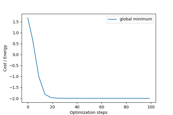
The minimum energy is -2 for the spin configuration \([s_1, s_2, s_3] = [1, 1, -1]\) which corresponds to \((\phi, \theta, \omega) = (0, 0, 0)\) for the second spin and \((\phi, \theta, \omega) = (0, \pi, 0)\) for the third spin. Note that gradient descent optimization might not find this global minimum due to the non-convex cost function, as is shown in the next section.
p1_final, p2_final = opt.param_groups[0]["params"]
print("Optimized angles:")
print(p1_final)
print(p2_final)
print("Final cost after optimization:")
print(cost(p1_final, p2_final))
Out:
Optimized angles:
tensor([1.9632e+00, 2.3284e-09, 2.3277e+00], dtype=torch.float64,
       requires_grad=True)
tensor([0.6521, 3.1416, 2.4300], dtype=torch.float64, requires_grad=True)
Final cost after optimization:
tensor(-2.0000, dtype=torch.float64, grad_fn=<SubBackward0>)
import matplotlib
import matplotlib.pyplot as plt

fig = plt.figure(figsize=(6, 4))

# Enable processing the Torch trainable tensors
with torch.no_grad():
    plt.plot(x, cost_pt, label = 'global minimum')
    plt.xlabel("Optimization steps")
    plt.ylabel("Cost / Energy")
    plt.legend()
    plt.show()
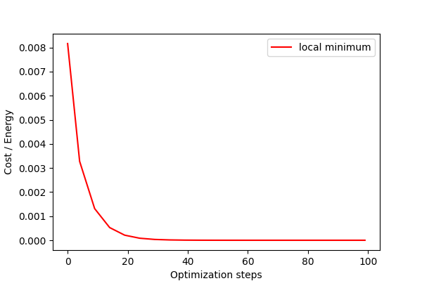
Local minimum
If the spins are initialized close to the local minimum of zero energy, the optimizer is likely to get stuck here and never find the global minimum at -2.
torch.manual_seed(9)
p3 = Variable((np.pi*torch.rand(3, dtype = torch.float64)), requires_grad = True)
p4 = Variable((np.pi*torch.rand(3, dtype = torch.float64)), requires_grad = True)

var_init_loc = [p3, p4]
cost_init_loc = cost(p3, p4)

print("Corresponding cost before optimization:")
print(cost_init_loc)
Out:
Corresponding cost before optimization:
tensor(0.0082, dtype=torch.float64, grad_fn=<SubBackward0>)
opt = torch.optim.SGD(var_init_loc, lr = 0.1)

def closure():
    opt.zero_grad()
    loss = cost(p3, p4)
    loss.backward()
    return loss

var_pt_loc = [var_init_loc]
cost_pt_loc = [cost_init_loc]

for j in range(100):
    opt.step(closure)
    if (j + 1) % 5 == 0:
        p3n, p4n = opt.param_groups[0]['params']
        costn = cost(p3n, p4n)
        var_pt_loc.append([p3n, p4n])
        cost_pt_loc.append(costn)

        # for clarity, the angles are printed as numpy arrays
        print('Energy after step {:5d}: {: .7f} | Angles: {}'.format(
            j+1, costn, [p3n.detach().numpy(), p4n.detach().numpy()]),"\n"
        )
Out:
Energy after step     5:  0.0032761 | Angles: [array([0.77369911, 2.63471297, 1.07981163]), array([0.26038622, 0.08659858, 1.91060734])]

Energy after step    10:  0.0013137 | Angles: [array([0.77369911, 2.63406019, 1.07981163]), array([0.26038622, 0.05483683, 1.91060734])]

Energy after step    15:  0.0005266 | Angles: [array([0.77369911, 2.63379816, 1.07981163]), array([0.26038622, 0.03471974, 1.91060734])]

Energy after step    20:  0.0002111 | Angles: [array([0.77369911, 2.63369307, 1.07981163]), array([0.26038622, 0.02198151, 1.91060734])]

Energy after step    25:  0.0000846 | Angles: [array([0.77369911, 2.63365094, 1.07981163]), array([0.26038622, 0.01391648, 1.91060734])]

Energy after step    30:  0.0000339 | Angles: [array([0.77369911, 2.63363405, 1.07981163]), array([0.26038622, 0.00881044, 1.91060734])]

Energy after step    35:  0.0000136 | Angles: [array([0.77369911, 2.63362729, 1.07981163]), array([0.26038622, 0.00557782, 1.91060734])]

Energy after step    40:  0.0000054 | Angles: [array([0.77369911, 2.63362457, 1.07981163]), array([0.26038622, 0.00353126, 1.91060734])]

Energy after step    45:  0.0000022 | Angles: [array([0.77369911, 2.63362348, 1.07981163]), array([0.26038622, 0.00223561, 1.91060734])]

Energy after step    50:  0.0000009 | Angles: [array([0.77369911, 2.63362305, 1.07981163]), array([2.60386222e-01, 1.41534339e-03, 1.91060734e+00])]

Energy after step    55:  0.0000004 | Angles: [array([0.77369911, 2.63362287, 1.07981163]), array([2.60386222e-01, 8.96040252e-04, 1.91060734e+00])]

Energy after step    60:  0.0000001 | Angles: [array([0.77369911, 2.6336228 , 1.07981163]), array([2.60386222e-01, 5.67274421e-04, 1.91060734e+00])]

Energy after step    65:  0.0000001 | Angles: [array([0.77369911, 2.63362278, 1.07981163]), array([2.60386222e-01, 3.59135947e-04, 1.91060734e+00])]

Energy after step    70:  0.0000000 | Angles: [array([0.77369911, 2.63362276, 1.07981163]), array([2.60386222e-01, 2.27365491e-04, 1.91060734e+00])]

Energy after step    75:  0.0000000 | Angles: [array([0.77369911, 2.63362276, 1.07981163]), array([2.60386222e-01, 1.43942891e-04, 1.91060734e+00])]

Energy after step    80:  0.0000000 | Angles: [array([0.77369911, 2.63362276, 1.07981163]), array([2.60386222e-01, 9.11288509e-05, 1.91060734e+00])]

Energy after step    85:  0.0000000 | Angles: [array([0.77369911, 2.63362276, 1.07981163]), array([2.60386222e-01, 5.76927932e-05, 1.91060734e+00])]

Energy after step    90:  0.0000000 | Angles: [array([0.77369911, 2.63362276, 1.07981163]), array([2.60386222e-01, 3.65247488e-05, 1.91060734e+00])]

Energy after step    95:  0.0000000 | Angles: [array([0.77369911, 2.63362276, 1.07981163]), array([2.60386222e-01, 2.31234648e-05, 1.91060734e+00])]

Energy after step   100:  0.0000000 | Angles: [array([0.77369911, 2.63362276, 1.07981163]), array([2.60386222e-01, 1.46392417e-05, 1.91060734e+00])]
fig = plt.figure(figsize=(6, 4))

# Enable processing the Torch trainable tensors
with torch.no_grad():
    plt.plot(x, cost_pt_loc, 'r', label = 'local minimum')
    plt.xlabel("Optimization steps")
    plt.ylabel("Cost / Energy")
    plt.legend()
    plt.show()
Try it yourself! Download and run this file with different initialization parameters and see how the results change.
Further reading
1. Maria Schuld and Francesco Petruccione. “Supervised Learning with Quantum Computers.” Springer, 2018.
2. Andrew Lucas. “Ising formulations of many NP problems.” arXiv:1302.5843, 2014.
3. Gary Kochenberger et al. “The Unconstrained Binary Quadratic Programming Problem: A Survey.” Journal of Combinatorial Optimization, 2014.