Quantum volume

Author: Olivia Di Matteo — Posted: 15 December 2020. Last updated: 15 April 2021.

Twice per year, a project called the TOP500 1 releases a list of the 500 most powerful supercomputing systems in the world. However, there is a large amount of variation in how supercomputers are built. They may run different operating systems and have varying amounts of memory. Some use 48-core processors, while others use processors with up to 260 cores. The speed of processors will differ, and they may be connected in different ways. We can’t rank them by simply counting the number of processors!

In order to make a fair comparison, we need benchmarking standards that give us a holistic view of their performance. To that end, the TOP500 rankings are based on something called the LINPACK benchmark 2. The task of the supercomputers is to solve a dense system of linear equations, and the metric of interest is the rate at which they perform floating-point operations (FLOPS). Today’s top machines reach speeds well into the regime of hundreds of petaFLOPS! While a single number certainly cannot tell the whole story, it still gives us insight into the quality of the machines, and provides a standard so we can compare them.

A similar problem is emerging with quantum computers: we can’t judge quantum computers on the number of qubits alone. Present-day devices have a number of limitations, an important one being gate error rates. Typically the qubits on a chip are not all connected to each other, so it may not be possible to perform operations on arbitrary pairs of them.

Considering this, can we tell if a machine with 20 noisy qubits is better than one with 5 very high-quality qubits? Or if a machine with 8 fully-connected qubits is better than one with 16 qubits of comparable error rate, but arranged in a square lattice? How can we make comparisons between different types of qubits?

Which of these qubit hardware graphs is the best?

To compare across all these facets, researchers have proposed a metric called “quantum volume” 3. Roughly, the quantum volume is a measure of the effective number of qubits a processor has. It is calculated by determining the largest number of qubits on which it can reliably run circuits of a prescribed type. You can think of it loosely as a quantum analogue of the LINPACK benchmark. Different quantum computers are tasked with solving the same problem, and the success will be a function of many properties: error rates, qubit connectivity, even the quality of the software stack. A single number won’t tell us everything about a quantum computer, but it does establish a framework for comparing them.

After working through this tutorial, you’ll be able to define quantum volume, explain the problem on which it’s based, and run the protocol to compute it!

Designing a benchmark for quantum computers

There are many different properties of a quantum computer that contribute to the successful execution of a computation. Therefore, we must be very explicit about what exactly we are benchmarking, and what is our measure of success. In general, to set up a benchmark for a quantum computer we need to decide on a number of things 4:

1. A family of circuits with a well-defined structure and variable size

2. A set of rules detailing how the circuits can be compiled

3. A measure of success for individual circuits

4. A measure of success for the family of circuits

5. (Optional) An experimental design specifying how the circuits are to be run

We’ll work through this list in order to see how the protocol for computing quantum volume fits within this framework.

The circuits

Quantum volume relates to the largest square circuit that a quantum processor can run reliably. This benchmark uses random square circuits with a very particular form:

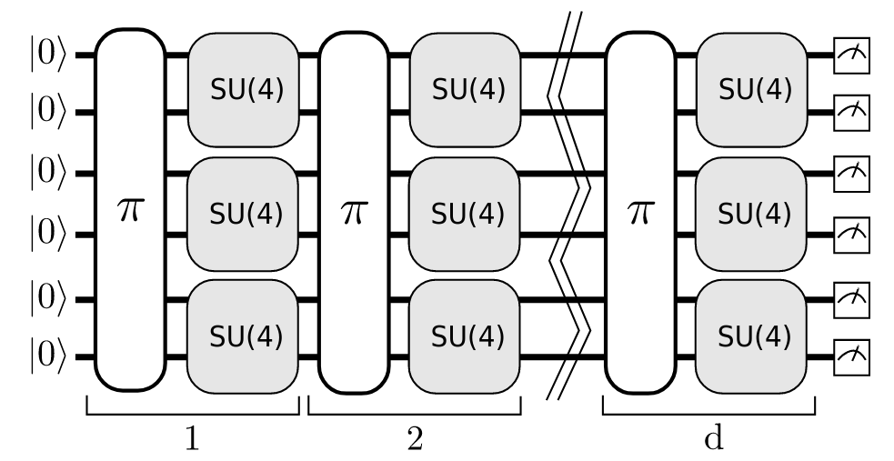
A schematic of the random circuit structure used in the quantum volume protocol. Image source: 3.

Specifically, the circuits consist of \(d\) sequential layers acting on \(d\) qubits. Each layer consists of two parts: a random permutation of the qubits, followed by Haar-random SU(4) operations performed on neighbouring pairs of qubits. (When the number of qubits is odd, the bottom-most qubit is idle while the SU(4) operations run on the pairs. However, it will still be incorporated by way of the permutations.) These circuits satisfy the criteria in item 1 — they have well-defined structure, and it is clear how they can be scaled to different sizes.

As for the compilation rules of item 2, to compute quantum volume we’re allowed to do essentially anything we’d like to the circuits in order to improve them. This includes optimization, hardware-aware considerations such as qubit placement and routing, and even resynthesis by finding unitaries that are close to the target, but easier to implement on the hardware 3.

Both the circuit structure and the compilation highlight how quantum volume is about more than just the number of qubits. The error rates will affect the achievable depth, and the qubit connectivity contributes through the layers of permutations because a very well-connected processor will be able to implement these in fewer steps than a less-connected one. Even the quality of the software and the compiler plays a role here: higher-quality compilers will produce circuits that fit better on the target devices, and will thus produce higher quality results.

The measures of success

Now that we have our circuits, we have to define the quantities that will indicate how well we’re able to run them. For that, we need a problem to solve. The problem used for computing quantum volume is called the heavy output generation problem. It has roots in the proposals for demonstrating quantum advantage 5. Many such proposals make use of the properties of various random quantum circuit families, as the distribution of the measurement outcomes may not be easy to sample using classical techniques.

A distribution that is theorized to fulfill this property is the distribution of heavy output bit strings. Heavy bit strings are those whose outcome probabilities are above the median of the distribution. For example, suppose we run a two-qubit circuit and find that the measurement probabilities for the output states are as follows:

measurement_probs = {"00": 0.558, "01": 0.182, "10": 0.234, "11": 0.026}

The median of this probability distribution is:

import numpy as np
prob_array = np.fromiter(measurement_probs.values(), dtype=np.float64)
print(f"Median = {np.median(prob_array):.3f}")

Out:

Median = 0.208

This means that the heavy bit strings are ‘00’ and ‘10’, because these are the two probabilities above the median. If we were to run this circuit, the probability of obtaining one of the heavy outputs is:

heavy_output_prob = np.sum(prob_array[prob_array > np.median(prob_array)])
print(f"Heavy output probability = {heavy_output_prob}")

Out:

Heavy output probability = 0.792

Each circuit in a circuit family has its own heavy output probability. If our quantum computer is of high quality, then we should expect to see heavy outputs quite often across all the circuits. On the other hand, if it’s of poor quality and everything is totally decohered, we will end up with output probabilities that are roughly all the same, as noise will reduce the probabilities to the uniform distribution.

The heavy output generation problem quantifies this — for our family of random circuits, do we obtain heavy outputs at least 2/3 of the time on average? Furthermore, do we obtain this with high confidence? This is the basis for quantum volume. Looking back at the criteria for our benchmarks, for item 3 the measure of success for each circuit is how often we obtain heavy outputs when we run the circuit and take a measurement. For item 4 the measure of success for the whole family is whether or not the mean of these probabilities is greater than 2/3 with high confidence.

On a related note, it is important to determine what heavy output probability we should expect to see on average. The intuition for how this can be calculated is as follows 5, 6. Suppose that our random square circuits scramble things up enough so that the effective operation looks like a Haar-random unitary \(U\). Since in the circuits we are applying \(U\) to the all-zero ket, the measurement outcome probabilities will be the moduli squared of the entries in the first column of \(U\).

Now if \(U\) is Haar-random, we can say something about the form of these entries. In particular, they are complex numbers for which both the real and imaginary parts are normally distributed with mean 0 and variance \(1/2^m\), where \(m\) is the number of qubits. Taking the modulus squared of such numbers and making a histogram yields a distribution of probabilities with the form \(\hbox{Pr}(p) \sim 2^m e^{-2^m p}.\) This is also known as the Porter-Thomas distribution.

By looking at the form of the underlying probability distribution, the exponential distribution \(\hbox{Pr}(x) = e^{-x}\), we can calculate some properties of the heavy output probabilities. First, we can integrate the exponential distribution to find that the median sits at \(\ln 2\). We can further compute the expectation value of obtaining something greater than the median by integrating \(x e^{-x}\) from \(\ln 2\) to \(\infty\) to obtain \((1 + \ln 2)/2\). This is the expected heavy output probability! Numerically it is around 0.85, as we will observe later in our results.

The benchmark

Now that we have our circuits and our measures of success, we’re ready to define the quantum volume.

Definition

The quantum volume \(V_Q\) of an \(n\)-qubit processor is defined as 3

\[\log_2(V_Q) = \hbox{argmax}_m \min (m, d(m))\]

where \(m \leq n\) is a number of qubits, and \(d(m)\) is the number of qubits in the largest square circuits for which we can reliably sample heavy outputs with probability greater than 2/3.

To see this more concretely, suppose we have a 20-qubit device and find that we get heavy outputs reliably for up to depth-4 circuits on any set of 4 qubits, then the quantum volume is \(\log_2 V_Q = 4\). Quantum volume is incremental, as shown below — we gradually work our way up to larger circuits, until we find something we can’t do. Very loosely, quantum volume is like an effective number of qubits. Even if we have those 20 qubits, only groups of up to 4 of them work well enough together to sample from distributions that would be considered hard.

This quantum computer has \(\log_2 V_Q = 4\), as the 4-qubit square circuits are the largest ones it can run successfully.

The maximum achieved quantum volume has been doubling at an increasing rate. In late 2020, the most recent announcements have been \(\log_2 V_Q = 6\) on IBM’s 27-qubit superconducting device ibmq_montreal 7, and \(\log_2 V_Q = 7\) on a Honeywell trapped-ion qubit processor 8. A device with an expected quantum volume of \(\log_2 V_Q = 22\) has also been announced by IonQ 9, though benchmarking results have not yet been published.

Note

In many sources, the quantum volume of processors is reported as \(V_Q\) explicitly, rather than \(\log_2 V_Q\) as is the convention in this demo. As such, IonQ’s processor has the potential for a quantum volume of \(2^{22} > 4000000\). Here we use the \(\log\) because it is more straightforward to understand that they have 22 high-quality, well-connected qubits than to extract this at first glance from the explicit value of the volume.

Computing the quantum volume

Equipped with our definition of quantum volume, it’s time to compute it ourselves! We’ll use the PennyLane-Qiskit plugin to compute the volume of a simulated version of one of the IBM processors, since their properties are easily accessible through this plugin.

Loosely, the protocol for quantum volume consists of three steps:

1. Construct random square circuits of increasing size

2. Run those circuits on both a simulator and on a noisy hardware device

3. Perform a statistical analysis of the results to determine what size circuits the device can run reliably

The largest reliable size will become the \(m\) in the expression for quantum volume.

Step 1: construct random square circuits

Recall that the structure of the circuits above is alternating layers of permutations and random SU(4) operations on pairs of qubits. Let’s implement the generation of such circuits in PennyLane.

First we write a function that randomly permutes qubits. We’ll do this by using numpy to generate a permutation, and then apply it with the built-in Permute() subroutine.

import pennylane as qml

# Object for random number generation from numpy
rng = np.random.default_rng()

def permute_qubits(num_qubits):
    # A random permutation
    perm_order = list(rng.permutation(num_qubits))
    qml.Permute(perm_order, wires=list(range(num_qubits)))

Next, we need to apply SU(4) gates to pairs of qubits. PennyLane doesn’t have built-in functionality to generate these random matrices, however its cousin Strawberry Fields does! We will use the random_interferometer method, which can generate unitary matrices uniformly at random. This function actually generates elements of U(4), but they are essentially equivalent up to a global phase.

from strawberryfields.utils import random_interferometer

def apply_random_su4_layer(num_qubits):
    for qubit_idx in range(0, num_qubits, 2):
        if qubit_idx < num_qubits - 1:
            rand_haar_su4 = random_interferometer(N=4)
            qml.QubitUnitary(rand_haar_su4, wires=[qubit_idx, qubit_idx + 1])

Next, let’s write a layering method to put the two together — this is just for convenience and to highlight the fact that these two methods together make up one layer of the circuit depth.

def qv_circuit_layer(num_qubits):
    permute_qubits(num_qubits)
    apply_random_su4_layer(num_qubits)

Let’s take a look! We’ll set up an ideal device with 5 qubits, and generate a circuit with 3 qubits. In this demo, we’ll work explicitly with quantum tapes since they are not immediately tied to a device. This will be convenient later when we need to run the same random circuit on two devices independently.

num_qubits = 5
dev_ideal = qml.device("lightning.qubit", shots=None, wires=num_qubits)

m = 3  # number of qubits

with qml.tape.QuantumTape() as tape:
    qml.layer(qv_circuit_layer, m, num_qubits=m)

expanded_tape = tape.expand(stop_at=lambda op: isinstance(op, qml.QubitUnitary))
print(qml.drawer.tape_text(expanded_tape, wire_order=dev_ideal.wires, show_all_wires=True, show_matrices=True))

Out:

0: ─╭SWAP───────╭U(M0)─╭SWAP───────╭U(M1)─╭U(M2)─┤
1: ─│─────╭SWAP─╰U(M0)─╰SWAP─╭SWAP─╰U(M1)─╰U(M2)─┤
2: ─╰SWAP─╰SWAP──────────────╰SWAP───────────────┤
3: ──────────────────────────────────────────────┤
4: ──────────────────────────────────────────────┤
M0 =
[[ 0.22234537+0.12795769j  0.24613682-0.34470179j  0.58179809-0.36478045j
  -0.16337007-0.50650086j]
 [-0.08840637-0.42456216j -0.01961572+0.35189839j  0.4214659 +0.31514336j
  -0.63733039+0.06764003j]
 [ 0.28919627-0.23577761j -0.11249786-0.67687982j  0.22914826+0.37205064j
   0.12755164+0.42749545j]
 [ 0.59999195+0.49689511j -0.29294024+0.37382355j  0.23724315-0.06544043j
  -0.039832  +0.3246437j ]]
M1 =
[[ 0.11583153-0.3628563j   0.55797708+0.48315028j -0.22400838-0.264741j
  -0.34856401+0.26149824j]
 [-0.04549494-0.25884483j  0.00258749-0.20351027j -0.26326583-0.70408962j
   0.33442905-0.46109931j]
 [-0.46824254-0.14274112j -0.00491681+0.61278881j -0.02506472+0.26582603j
   0.54135395-0.14312156j]
 [ 0.73672445-0.05881259j  0.19534118+0.01057264j -0.29145879+0.398047j
   0.33955583-0.23837031j]]
M2 =
[[-0.33352575+0.21982221j -0.29128941-0.51347253j  0.63543764-0.11913356j
   0.27186717+0.00704727j]
 [-0.22330473+0.02289549j  0.1997405 -0.47316218j -0.23040621-0.14078015j
  -0.47922028-0.61909121j]
 [-0.00705247+0.82724695j  0.52220719+0.02527864j -0.05490671-0.04899343j
   0.03167901+0.18935341j]
 [ 0.23396138-0.22566431j  0.32400589+0.09694607j  0.54666955-0.45261179j
  -0.48177768+0.2101061j ]]

The first thing to note is that the last two qubits are never used in the operations, since the quantum volume circuits are square. Another important point is that this circuit with 3 layers actually has depth much greater than 3, since each layer has both SWAPs and SU(4) operations that are further decomposed into elementary gates when run on the actual processor.

One last thing we’ll need before running our circuits is the machinery to determine the heavy outputs. This is quite an interesting aspect of the protocol — we’re required to compute the heavy outputs classically in order to get the results! As a consequence, it will only be possible to calculate quantum volume for processors up to a certain point before they become too large.

That said, classical simulators are always improving, and can simulate circuits with numbers of qubits well into the double digits (though they may need a supercomputer to do so). Furthermore, the designers of the protocol don’t expect this to be an issue until gate error rates decrease below \(\approx 10^{-4}\), after which we may need to make adjustments to remove the classical simulation, or even consider new volume metrics 3.

The heavy outputs can be retrieved from a classically-obtained probability distribution as follows:

def heavy_output_set(m, probs):
    # Compute heavy outputs of an m-qubit circuit with measurement outcome
    # probabilities given by probs, which is an array with the probabilities
    # ordered as '000', '001', ... '111'.

    # Sort the probabilities so that those above the median are in the second half
    probs_ascending_order = np.argsort(probs)
    sorted_probs = probs[probs_ascending_order]

    # Heavy outputs are the bit strings above the median
    heavy_outputs = [
        # Convert integer indices to m-bit binary strings
        format(x, f"#0{m+2}b")[2:] for x in list(probs_ascending_order[2 ** (m - 1) :])
    ]

    # Probability of a heavy output
    prob_heavy_output = np.sum(sorted_probs[2 ** (m - 1) :])

    return heavy_outputs, prob_heavy_output

As an example, let’s compute the heavy outputs and probability for our circuit above.

# Adds a measurement of the first m qubits to the previous circuit
with tape:
    qml.probs(wires=range(m))

# Run the circuit, compute heavy outputs, and print results
output_probs = qml.execute([tape], dev_ideal, None)  # returns a list of result !
output_probs = output_probs[0].reshape(2 ** m, )
heavy_outputs, prob_heavy_output = heavy_output_set(m, output_probs)

print("State\tProbability")
for idx, prob in enumerate(output_probs):
    bit_string = format(idx, f"#05b")[2:]
    print(f"{bit_string}\t{prob:.4f}")

print(f"\nMedian is {np.median(output_probs):.4f}")
print(f"Probability of a heavy output is {prob_heavy_output:.4f}")
print(f"Heavy outputs are {heavy_outputs}")

Out:

State     Probability
000           0.0559
001           0.3687
010           0.0326
011           0.0179
100           0.0550
101           0.3590
110           0.1103
111           0.0005

Median is 0.0554
Probability of a heavy output is 0.8939
Heavy outputs are ['000', '110', '101', '001']

Step 2: run the circuits

Now it’s time to run the protocol. First, let’s set up our hardware device. We’ll use a simulated version of the 5-qubit IBM Lima as an example — the reported quantum volume according to IBM is \(V_Q=8\), so we endeavour to reproduce that here. This means that we should be able to run our square circuits reliably on up to \(\log_2 V_Q =3\) qubits.

Note

In order to access the IBM Q backend, users must have an IBM Q account configured. This can be done by running:

from qiskit import IBMQ
IBMQ.save_account('MY_API_TOKEN')

A token can be generated by logging into your IBM Q account here .

Note

Users can get a list of available IBM Q backends by importing IBM Q, specifying their provider and then calling: provider.backends()

dev_lima = qml.device("qiskit.ibmq", wires=5, backend="ibmq_lima")

First, we can take a look at the arrangement of the qubits on the processor by plotting its hardware graph.

import matplotlib.pyplot as plt
import networkx as nx

lima_hardware_graph = nx.Graph(dev_lima.backend.configuration().coupling_map)

nx.draw_networkx(
    lima_hardware_graph,
    node_color="cyan",
    labels={x: x for x in range(dev_lima.num_wires)},
)

This hardware graph is not fully connected, so the quantum compiler will have to make some adjustments when non-connected qubits need to interact.

To actually perform the simulations, we’ll need to access a copy of the Lima noise model. Again, we won’t be running on Lima directly — we’ll set up a local device to simulate its behaviour.

from qiskit.providers.aer import noise

noise_model = noise.NoiseModel.from_backend(dev_lima.backend)

dev_noisy = qml.device(
    "qiskit.aer", wires=dev_lima.num_wires, shots=1000, noise_model=noise_model
)

As a final point, since we are allowed to do as much optimization as we like, let’s put the compiler to work. The compiler will perform a number of optimizations to simplify our circuit. We’ll also specify some high-quality qubit placement and routing techniques 10 in order to fit the circuits on the hardware graph in the best way possible.

coupling_map = dev_lima.backend.configuration().to_dict()["coupling_map"]

dev_noisy.set_transpile_args(
    **{
        "optimization_level": 3,
        "coupling_map": coupling_map,
        "layout_method": "sabre",
        "routing_method": "sabre",
    }
)

Let’s run the protocol. We’ll start with the smallest circuits on 2 qubits, and make our way up to 5. At each \(m\), we’ll look at 200 randomly generated circuits.

min_m = 2
max_m = 5
num_ms = (max_m - min_m) + 1

num_trials = 200

# To store the results
probs_ideal = np.zeros((num_ms, num_trials))
probs_noisy = np.zeros((num_ms, num_trials))

for m in range(min_m, max_m + 1):
    for trial in range(num_trials):

        # Simulate the circuit analytically
        with qml.tape.QuantumTape() as tape:
            qml.layer(qv_circuit_layer, m, num_qubits=m)
            qml.probs(wires=range(m))

        output_probs = qml.execute([tape], dev_ideal, None)
        output_probs = output_probs[0].reshape(2 ** m, )
        heavy_outputs, prob_heavy_output = heavy_output_set(m, output_probs)

        # Execute circuit on the noisy device
        qml.execute([tape], dev_noisy, None)

        # Get the output bit strings; flip ordering of qubits to match PennyLane
        counts = dev_noisy._current_job.result().get_counts()
        reordered_counts = {x[::-1]: counts[x] for x in counts.keys()}

        device_heavy_outputs = np.sum(
            [
                reordered_counts[x] if x[:m] in heavy_outputs else 0
                for x in reordered_counts.keys()
            ]
        )
        fraction_device_heavy_output = device_heavy_outputs / dev_noisy.shots

        probs_ideal[m - min_m, trial] = prob_heavy_output
        probs_noisy[m - min_m, trial] = fraction_device_heavy_output

Step 3: perform a statistical analysis

Having run our experiments, we can now get to the heart of the quantum volume protocol: what is the largest square circuit that our processor can run? Let’s first check out the means and see how much higher they are than 2/3.

probs_mean_ideal = np.mean(probs_ideal, axis=1)
probs_mean_noisy = np.mean(probs_noisy, axis=1)

print(f"Ideal mean probabilities:")
for idx, prob in enumerate(probs_mean_ideal):
    print(f"m = {idx + min_m}: {prob:.6f} {'above' if prob > 2/3 else 'below'} threshold.")

print(f"\nDevice mean probabilities:")
for idx, prob in enumerate(probs_mean_noisy):
    print(f"m = {idx + min_m}: {prob:.6f} {'above' if prob > 2/3 else 'below'} threshold.")

Out:

Ideal mean probabilities:
m = 2: 0.801480 above threshold.
m = 3: 0.853320 above threshold.
m = 4: 0.832995 above threshold.
m = 5: 0.858370 above threshold.

Device mean probabilities:
m = 2: 0.765920 above threshold.
m = 3: 0.773985 above threshold.
m = 4: 0.674380 above threshold.
m = 5: 0.639500 below threshold.

We see that the ideal probabilities are well over 2/3. In fact, they’re quite close to the expected value of \((1 + \ln 2)/2\), which we recall from above is \(\approx 0.85\). For this experiment, we see that the device probabilities are also above the threshold (except one). But it isn’t enough that just the mean of the heavy output probabilities is greater than 2/3. Since we’re dealing with randomness, we also want to ensure these results were not just a fluke! To be confident, we also want to be above 2/3 within 2 standard deviations \((\sigma)\) of the mean. This is referred to as a 97.5% confidence interval (since roughly 97.5% of a normal distribution sits within \(2\sigma\) of the mean.)

At this point, we’re going to do some statistical sorcery and make some assumptions about our distributions. Whether or not a circuit is successful (in the sense that it produces heavy outputs more the 2/3 of the time) is a binary outcome. When we sample many circuits, it is almost like we are sampling from a binomial distribution where the outcome probability is equivalent to the heavy output probability. In the limit of a large number of samples (in this case 200 circuits), a binomial distribution starts to look like a normal distribution. If we make this approximation, we can compute the standard deviation and use it to make our confidence interval. With the normal approximation, the standard deviation is

\[\sigma = \sqrt{\frac{p_h(1 - p_h)}{N}},\]

where \(p_h\) is the average heavy output probability, and \(N\) is the number of circuits.

stds_ideal = np.sqrt(probs_mean_ideal * (1 - probs_mean_ideal) / num_trials)
stds_noisy = np.sqrt(probs_mean_noisy * (1 - probs_mean_noisy) / num_trials)

Now that we have our standard deviations, let’s see if our means are at least \(2\sigma\) away from the threshold!

fig, ax = plt.subplots(2, 2, sharex=True, sharey=True, figsize=(9, 6))
ax = ax.ravel()

for m in range(min_m - 2, max_m + 1 - 2):
    ax[m].hist(probs_noisy[m, :])
    ax[m].set_title(f"m = {m + min_m}", fontsize=16)
    ax[m].set_xlabel("Heavy output probability", fontsize=14)
    ax[m].set_ylabel("Occurrences", fontsize=14)
    ax[m].axvline(x=2.0 / 3, color="black", label="2/3")
    ax[m].axvline(x=probs_mean_noisy[m], color="red", label="Mean")
    ax[m].axvline(
        x=(probs_mean_noisy[m] - 2 * stds_noisy[m]),
        color="red",
        linestyle="dashed",
        label="2σ",
    )

fig.suptitle("Heavy output distributions for (simulated) Lima QPU", fontsize=18)
plt.legend(fontsize=14)
plt.tight_layout()

Let’s verify this numerically:

two_sigma_below = probs_mean_noisy - 2 * stds_noisy

for idx, prob in enumerate(two_sigma_below):
    print(f"m = {idx + min_m}: {prob:.6f} {'above' if prob > 2/3 else 'below'} threshold.")

Out:

m = 2: 0.706039 above threshold.
m = 3: 0.714836 above threshold.
m = 4: 0.608109 below threshold.
m = 5: 0.571597 below threshold.

We see that we are \(2\sigma\) above the threshold only for \(m=2\), and \(m=3\). Thus, we find that the quantum volume of our simulated Lima is \(\log_2 V_Q = 3\), or \(V_Q = 8\), as expected.

This framework and code will allow you to calculate the quantum volume of many different processors. Try it yourself! What happens if we don’t specify a large amount of compiler optimization? How does the volume compare across different hardware devices? You can even build your own device configurations and noise models to explore the extent to which different factors affect the volume.

Concluding thoughts

Quantum volume is a metric used for comparing the quality of different quantum computers. By determining the largest square random circuits a processor can run reliably, it provides a measure of the effective number of qubits a processor has. Furthermore, it goes beyond just gauging quality by a number of qubits — it incorporates many different aspects of a device such as its compiler, qubit connectivity, and gate error rates.

However, as with any benchmark, it is not without limitations. A key one already discussed is that the heavy output generation problem requires us to simulate circuits classically in addition to running them on a device. While this is perhaps not an issue now, it will surely become one in the future. The number of qubits continues to increase and error rates are getting lower, both of which imply that our square circuits will be growing in both width and depth as time goes on. Eventually they will reach a point where they are no longer classical simulable, and we will have to design new benchmarks.

Another limitation is that the protocol only looks at one type of circuit, i.e., square circuits. It might be the case that a processor has very few qubits, but also very low error rates. For example, what if a processor with 5 qubits can run circuits with up to 20 layers? Quantum volume would limit us to \(\log_2 V_Q = 5\) and the high quality of those qubits is not reflected in this. To that end, a more general volumetric benchmark framework was proposed that includes not only square circuits, but also rectangular circuits 4. Investigating very deep circuits on few qubits (and very shallow circuits on many qubits) will give us a broader overview of a processor’s quality. Furthermore, the flexibility of the framework of 4 will surely inspire us to create new types of benchmarks. Having a variety of benchmarks calculated in different ways is beneficial and gives us a broader view of the performance of quantum computers.

References

1

https://www.top500.org/

2

https://www.top500.org/project/linpack/

3(1,2,3,4,5)

Cross, A. W., Bishop, L. S., Sheldon, S., Nation, P. D., & Gambetta, J. M., Validating quantum computers using randomized model circuits, Physical Review A, 100(3), (2019).

4(1,2,3)

Blume-Kohout, R., & Young, K. C., A volumetric framework for quantum computer benchmarks, Quantum, 4, 362 (2020).

5(1,2)

Aaronson, S., & Chen, L., Complexity-theoretic foundations of quantum supremacy experiments. arXiv 1612.05903 quant-ph

6

O’Donnell, R. CMU course: Quantum Computation and Quantum Information 2018. Lecture 25

7

Jurcevic et al. Demonstration of quantum volume 64 on a superconducting quantum computing system. arXiv 2008.08571 quant-ph

8

https://www.honeywell.com/en-us/newsroom/news/2020/09/achieving-quantum-volume-128-on-the-honeywell-quantum-computer

9

https://www.prnewswire.com/news-releases/ionq-unveils-worlds-most-powerful-quantum-computer-301143782.html

10

Li, G., Ding, Y., & Xie, Y., Tackling the qubit mapping problem for nisq-era quantum devices, In Proceedings of the Twenty-Fourth International Conference on Architectural Support for Programming Languages and Operating Systems (pp. 1001–1014) (2019). New York, NY, USA: Association for Computing Machinery.

About the author

Olivia Di Matteo

Olivia is an Assistant Professor in the Department of Electrical and Computer Engineering at The University of British Columbia. Her research interests are quantum compilation, software, and algorithms.

demos/quantum_volume

 

Download Python script

 

Download Notebook

 

View on GitHub