Understanding the Haar measure

Author: Olivia Di Matteo — Posted: 22 March 2021. Last updated: 22 March 2021.

If you’ve ever dug into the literature about random quantum circuits, variational ansatz structure, or anything related to the structure and properties of unitary operations, you’ve likely come across a statement like the following: “Assume that \(U\) is sampled uniformly at random from the Haar measure”. In this demo, we’re going to unravel this cryptic statement and take an in-depth look at what it means. You’ll gain an understanding of the general concept of a measure, the Haar measure and its special properties, and you’ll learn how to sample from it using tools available in PennyLane and other scientific computing frameworks. By the end of this demo, you’ll be able to include that important statement in your own work with confidence!

Note

To get the most out of this demo, it is helpful if you are familiar with integration of multi-dimensional functions, the Bloch sphere, and the conceptual ideas behind decompositions and factorizations of unitary matrices (see, e.g., 4.5.1 and 4.5.2 of 1).

Measure

Measure theory is a branch of mathematics that studies things that are measurable—think length, area, or volume, but generalized to mathematical spaces and even higher dimensions. Loosely, the measure tells you about how “stuff” is distributed and concentrated in a mathematical set or space. An intuitive way to understand the measure is to think about a sphere. An arbitrary point on a sphere can be parametrized by three numbers—depending on what you’re doing, you may use Cartesian coordinates \((x, y, z)\), or it may be more convenient to use spherical coordinates \((\rho, \phi, \theta)\).

Suppose you wanted to compute the volume of a solid sphere with radius \(r\). This can be done by integrating over the three coordinates \(\rho, \phi\), and \(\theta\). Your first thought here may be to simply integrate each parameter over its full range, like so:

\[V = \int_0^{r} \int_0^{2\pi} \int_0^{\pi} d\rho~ d\phi~ d\theta = 2\pi^2 r\]

But, we know that the volume of a sphere of radius \(r\) is \(\frac{4}{3}\pi r^3\), so what we got from this integral is clearly wrong! Taking the integral naively like this doesn’t take into account the structure of the sphere with respect to the parameters. For example, consider two small, infinitesimal elements of area with the same difference in \(\theta\) and \(\phi\), but at different values of \(\theta\):

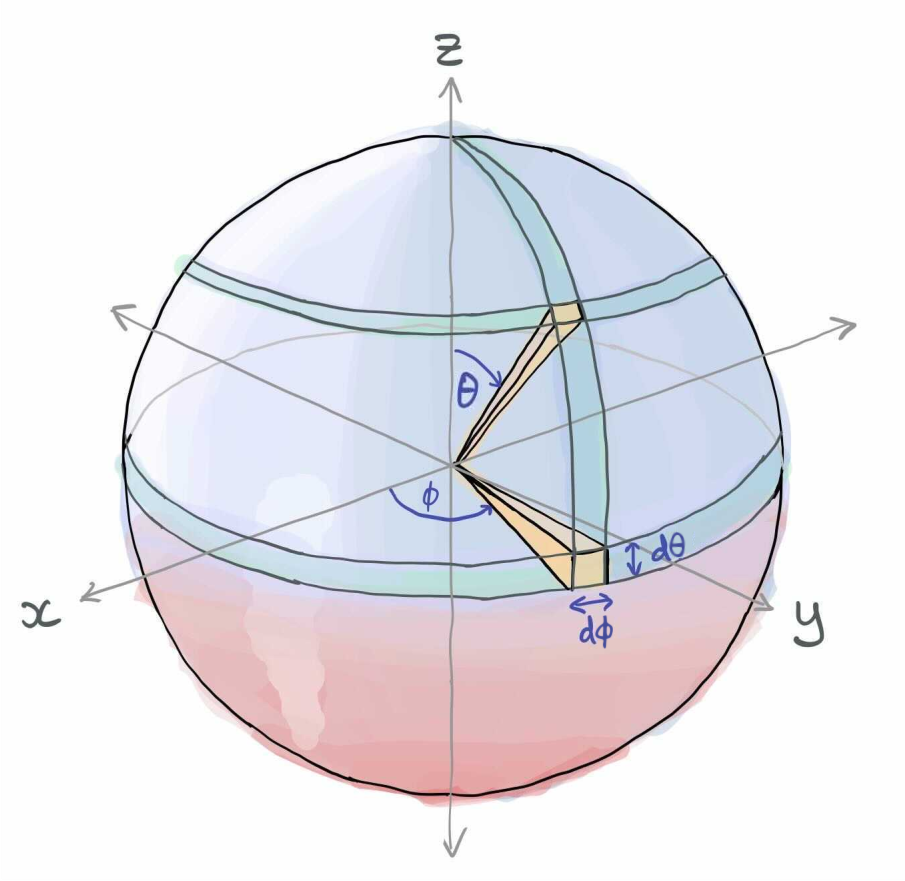
Even though the differences \(d\theta\) and \(d\phi\) themselves are the same, there is way more “stuff” near the equator of the sphere than there is near the poles. We must take into account the value of \(\theta\) when computing the integral! Specifically, we multiply by the function \(\sin\theta\)—the properties of the \(\sin\) function mean that the most weight will occur around the equator where \(\theta=\pi/2\), and the least weight near the poles where \(\theta=0\) and \(\theta=\pi\).

Similar care must be taken for \(\rho\). The contribution to volume of parts of the sphere with a large \(\rho\) is far more than for a small \(\rho\)—we should expect the contribution to be proportional to \(\rho^2\), given that the surface area of a sphere of radius \(r\) is \(4\pi r^2\).

On the other hand, for a fixed \(\rho\) and \(\theta\), the length of the \(d\phi\) is the same all around the circle. If put all these facts together, we find that the actual expression for the integral should look like this:

\[V = \int_0^r \int_0^{2\pi} \int_0^{\pi} \rho^2 \sin \theta~ d\rho~ d\phi~ d\theta = \frac{4}{3}\pi r^3\]

These extra terms that we had to add to the integral, \(\rho^2 \sin \theta\), constitute the measure. The measure weights portions of the sphere differently depending on where they are in the space. While we need to know the measure to properly integrate over the sphere, knowledge of the measure also gives us the means to perform another important task, that of sampling points in the space uniformly at random. We can’t simply sample each parameter from the uniform distribution over its domain—as we experienced already, this doesn’t take into account how the sphere is spread out over space. The measure describes the distribution of each parameter and gives a recipe for sampling them in order to obtain something properly uniform.

The Haar measure

Operations in quantum computing are described by unitary matrices. Unitary matrices, like points on a sphere, can be expressed in terms of a fixed set of coordinates, or parameters. For example, the most general single-qubit rotation implemented in PennyLane (Rot) is expressed in terms of three parameters like so,

\[\begin{split}U(\phi, \theta, \omega) = \begin{pmatrix} e^{-i(\phi + \omega)/2} \cos(\theta/2) & -e^{i(\phi - \omega)/2} \sin(\theta/2) \\ e^{-i(\phi - \omega)/2} \sin(\theta/2) & e^{i(\phi + \omega)/2} \cos(\theta/2) \end{pmatrix}.\end{split}\]

For every dimension \(N\), the unitary matrices of size \(N \times N\) constitute the unitary group \(U(N)\). We can perform operations on elements of this group, such as apply functions to them, integrate over them, or sample uniformly over them, just as we can do to points on a sphere. When we do such tasks with respect to the sphere, we have to add the measure in order to properly weight the different regions of space. The Haar measure provides the analogous terms we need for working with the unitary group.

For an \(N\)-dimensional system, the Haar measure, often denoted by \(\mu_N\), tells us how to weight the elements of \(U(N)\). For example, suppose \(f\) is a function that acts on elements of \(U(N)\), and we would like to take its integral over the group. We must write this integral with respect to the Haar measure, like so:

\[\int_{V \in U(N)} f(V) d\mu_N(V).\]

As with the measure term of the sphere, \(d\mu_N\) itself can be broken down into components depending on individual parameters. While the Haar measure can be defined for every dimension \(N\), the mathematical form gets quite hairy for larger dimensions—in general, an \(N\)-dimensional unitary requires at least \(N^2 - 1\) parameters, which is a lot to keep track of! Therefore we’ll start with the case of a single qubit \((N=2)\), then show how things generalize.

Single-qubit Haar measure

The single-qubit case provides a particularly nice entry point because we can continue our comparison to spheres by visualizing single-qubit states on the Bloch sphere. As expressed above, the measure provides a recipe for sampling elements of the unitary group in a properly uniform manner, given the structure of the group. One useful consequence of this is that it provides a method to sample quantum states uniformly at random—we simply generate Haar-random unitaries, and apply them to a fixed basis state such as \(\vert 0\rangle\).

We’ll see how this works in good time. First, we’ll take a look at what happens when we ignore the measure and do things wrong. Suppose we sample quantum states by applying unitaries obtained by the parametrization above, but sample the angles \(\omega, \phi\), and \(\theta\) from the flat uniform distribution between \([0, 2\pi)\) (fun fact: there is a measure implicit in this kind of sampling too! It just has a constant value, because each point is equally likely to be sampled).

import pennylane as qml
import numpy as np
import matplotlib.pyplot as plt

# set the random seed
np.random.seed(42)

# Use the mixed state simulator to save some steps in plotting later
dev = qml.device('default.mixed', wires=1)

@qml.qnode(dev)
def not_a_haar_random_unitary():
    # Sample all parameters from their flat uniform distribution
    phi, theta, omega = 2 * np.pi * np.random.uniform(size=3)
    qml.Rot(phi, theta, omega, wires=0)
    return qml.state()

num_samples = 2021

not_haar_samples = [not_a_haar_random_unitary() for _ in range(num_samples)]

In order to plot these on the Bloch sphere, we’ll need to do one more step, and convert the quantum states into Bloch vectors.

X = np.array([[0, 1], [1, 0]])
Y = np.array([[0, -1j], [1j, 0]])
Z = np.array([[1, 0], [0, -1]])

# Used the mixed state simulator so we could have the density matrix for this part!
def convert_to_bloch_vector(rho):
    """Convert a density matrix to a Bloch vector."""
    ax = np.trace(np.dot(rho, X)).real
    ay = np.trace(np.dot(rho, Y)).real
    az = np.trace(np.dot(rho, Z)).real
    return [ax, ay, az]

not_haar_bloch_vectors = np.array([convert_to_bloch_vector(s) for s in not_haar_samples])

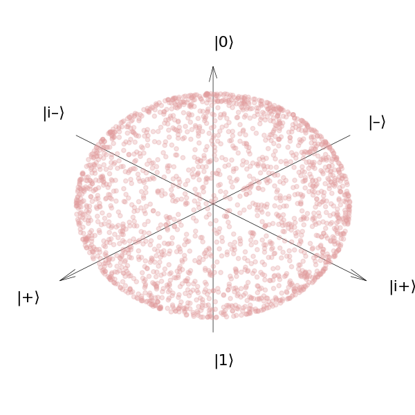
With this done, let’s find out where our “uniformly random” states ended up:

def plot_bloch_sphere(bloch_vectors):
    """ Helper function to plot vectors on a sphere."""
    fig = plt.figure(figsize=(6, 6))
    ax = fig.add_subplot(111, projection='3d')
    fig.subplots_adjust(left=0, right=1, bottom=0, top=1)

    ax.grid(False)
    ax.set_axis_off()
    ax.view_init(30, 45)
    ax.dist = 7

    # Draw the axes (source: https://github.com/matplotlib/matplotlib/issues/13575)
    x, y, z = np.array([[-1.5,0,0], [0,-1.5,0], [0,0,-1.5]])
    u, v, w = np.array([[3,0,0], [0,3,0], [0,0,3]])
    ax.quiver(x, y, z, u, v, w, arrow_length_ratio=0.05, color="black", linewidth=0.5)

    ax.text(0, 0, 1.7, r"|0⟩", color="black", fontsize=16)
    ax.text(0, 0, -1.9, r"|1⟩", color="black", fontsize=16)
    ax.text(1.9, 0, 0, r"|+⟩", color="black", fontsize=16)
    ax.text(-1.7, 0, 0, r"|–⟩", color="black", fontsize=16)
    ax.text(0, 1.7, 0, r"|i+⟩", color="black", fontsize=16)
    ax.text(0,-1.9, 0, r"|i–⟩", color="black", fontsize=16)

    ax.scatter(
        bloch_vectors[:,0], bloch_vectors[:,1], bloch_vectors[:, 2], c='#e29d9e', alpha=0.3
    )

plot_bloch_sphere(not_haar_bloch_vectors)

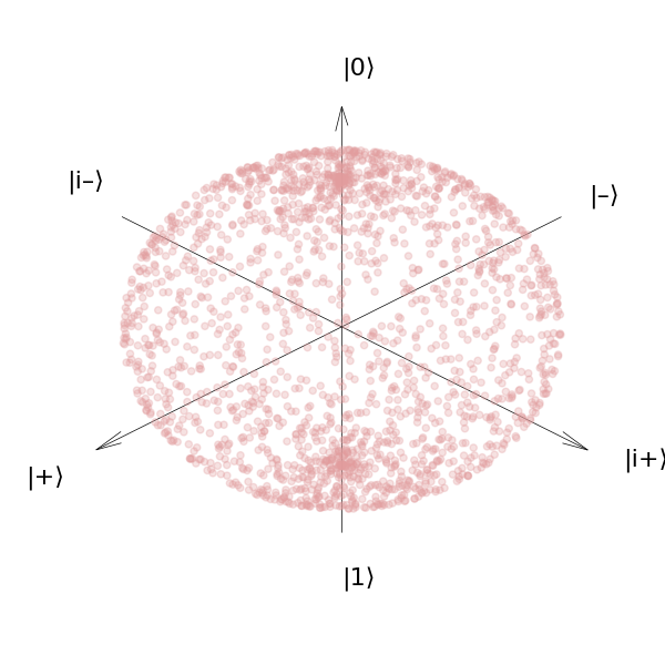
You can see from this plot that even though our parameters were sampled from a uniform distribution, there is a noticeable amount of clustering around the poles of the sphere. Despite the input parameters being uniform, the output is very much not uniform. Just like the regular sphere, the measure is larger near the equator, and if we just sample uniformly, we won’t end up populating that area as much. To take that into account we will need to sample from the proper Haar measure, and weight the different parameters appropriately.

For a single qubit, the Haar measure looks much like the case of a sphere, minus the radial component. Intuitively, all qubit state vectors have length 1, so it makes sense that this wouldn’t play a role here. The parameter that we will have to weight differently is \(\theta\), and in fact the adjustment in measure is identical to that we had to do with the polar axis of the sphere, i.e., \(\sin \theta\). In order to sample the \(\theta\) uniformly at random in this context, we must sample from the distribution \(\hbox{Pr}(\theta) = \sin \theta\). We can accomplish this by setting up a custom probability distribution with rv_continuous in scipy.

from scipy.stats import rv_continuous

class sin_prob_dist(rv_continuous):
    def _pdf(self, theta):
        # The 0.5 is so that the distribution is normalized
        return 0.5 * np.sin(theta)

# Samples of theta should be drawn from between 0 and pi
sin_sampler = sin_prob_dist(a=0, b=np.pi)

@qml.qnode(dev)
def haar_random_unitary():
    phi, omega = 2 * np.pi * np.random.uniform(size=2) # Sample phi and omega as normal
    theta = sin_sampler.rvs(size=1) # Sample theta from our new distribution
    qml.Rot(phi, theta, omega, wires=0)
    return qml.state()

haar_samples = [haar_random_unitary() for _ in range(num_samples)]
haar_bloch_vectors = np.array([convert_to_bloch_vector(s) for s in haar_samples])

plot_bloch_sphere(haar_bloch_vectors)

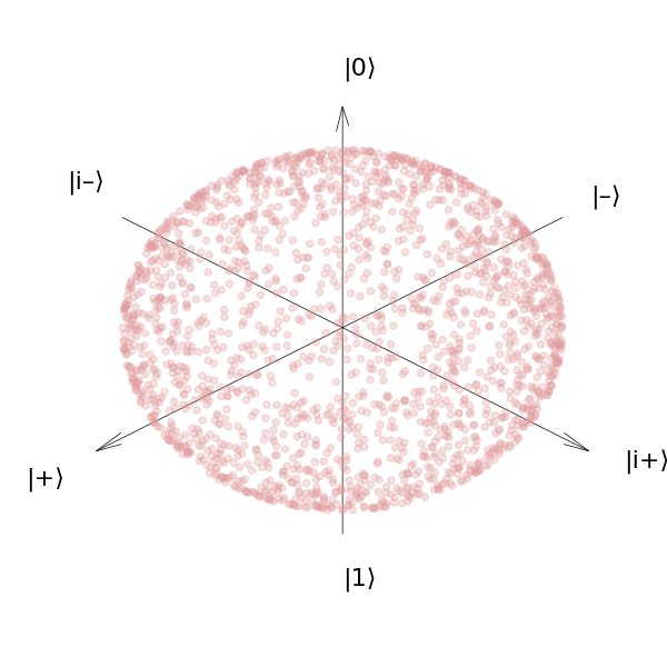
We see that when we use the correct measure, our qubit states are now much better distributed over the sphere. Putting this information together, we can now write the explicit form for the single-qubit Haar measure:

\[d\mu_2 = \sin \theta d\theta \cdot d\omega \cdot d\phi.\]

Show me more math!

While we can easily visualize the single-qubit case, this is no longer possible when we increase the number of qubits. Regardless, we can still obtain a mathematical expression for the Haar measure in arbitrary dimensions. In the previous section, we expressed the Haar measure in terms of a set of parameters that can be used to specify the unitary group \(U(2)\). Such a parametrization is not unique, and in fact there are multiple ways to factorize, or decompose an \(N\)-dimensional unitary operation into a set of parameters.

Many of these parametrizations come to us from the study of photonics. Here, arbitrary operations are broken down into elementary operations involving only a few parameters which correspond directly to parameters of the physical apparatus used to implement them (beamsplitters and phase shifts). Rather than qubits, such operations act on modes, or qumodes. They are expressed as elements of the \(N\)-dimensional special unitary group. This group, written as \(SU(N)\), is the continuous group consisting of all \(N \times N\) unitary operations with determinant 1 (essentially like \(U(N)\), minus a potential global phase).

Note

Elements of \(SU(N)\) and \(U(N)\) can still be considered as multi-qubit operations in the cases where \(N\) is a power of 2, but they must be translated from continuous-variable operations into qubit operations. (In PennyLane, this can be done by feeding the unitaries to the QubitUnitary operation directly. Alternatively, one can use quantum compilation to express the operations as a sequence of elementary gates such as Pauli rotations and CNOTs.)

Tip

If you haven’t had many opportunities to work in terms of qumodes, the Strawberry Fields documentation is a good starting point.

For example, we saw already above that for \(N=2\), we can write

\[\begin{split}U(\phi, \theta, \omega) = \begin{pmatrix} e^{-i(\phi + \omega)/2} \cos(\theta/2) & -e^{i(\phi - \omega)/2} \sin(\theta/2) \\ e^{-i(\phi - \omega)/2} \sin(\theta/2) & e^{i(\phi + \omega)/2} \cos(\theta/2) \end{pmatrix}.\end{split}\]

This unitary can be factorized as follows:

\[\begin{split}U(\phi, \theta, \omega) = \begin{pmatrix} e^{-i\omega/2} & 0 \\ 0 & e^{i\omega/2} \end{pmatrix} \begin{pmatrix} \cos(\theta/2) & -\sin(\theta/2) \\ \sin(\theta/2) & \cos(\theta/2) \end{pmatrix} \begin{pmatrix} e^{-i\phi/2} & 0 \\ 0 & e^{i\phi/2} \end{pmatrix}\end{split}\]

The middle operation is a beamsplitter; the other two operations are phase shifts. We saw earlier that for \(N=2\), \(d\mu_2 = \sin\theta d\theta d\omega d\phi\)—note how the parameter in the beamsplitter contributes to the measure in a different way than those of the phase shifts. As mentioned above, for larger values of \(N\) there are multiple ways to decompose the unitary. Such decompositions rewrite elements in \(SU(N)\) acting on \(N\) modes as a sequence of operations acting only on 2 modes, \(SU(2)\), and single-mode phase shifts. Shown below are three examples 2, 3, 4:

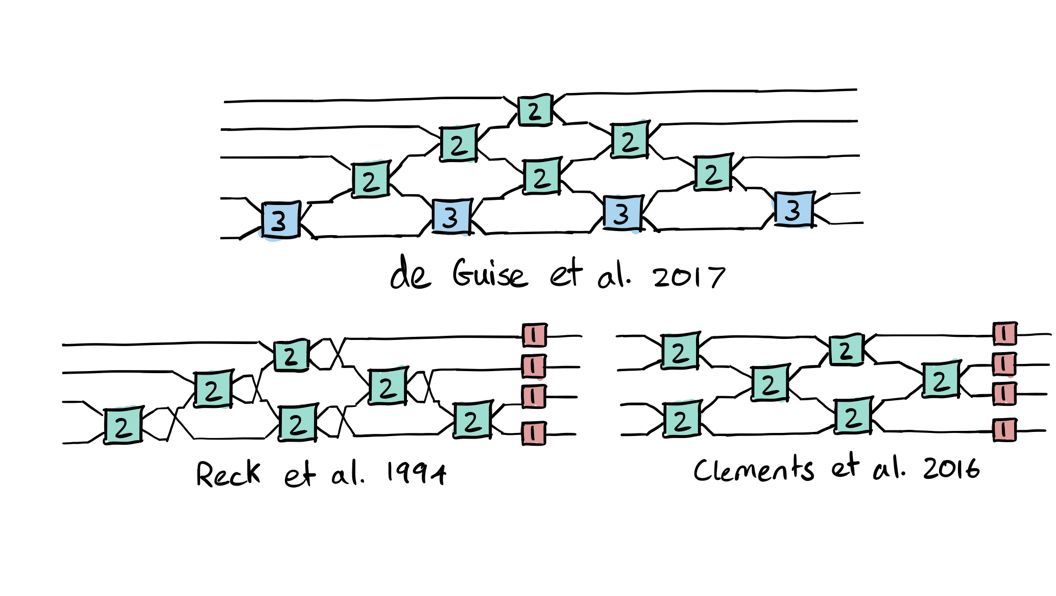
In these graphics, every wire is a different mode. Every box represents an operation on one or more modes, and the number in the box indicates the number of parameters. The boxes containing a 1 are simply phase shifts on individual modes. The blocks containing a 3 are \(SU(2)\) transforms with 3 parameters, such as the \(U(\phi, \theta, \omega)\) above. Those containing a 2 are \(SU(2)\) transforms on pairs of modes with 2 parameters, similar to the 3-parameter ones but with \(\omega = \phi\).

Although the decompositions all produce the same set of operations, their structure and parametrization may have consequences in practice. The first 2 has a particularly convenient form that leads to a recursive definition of the Haar measure. The decomposition is formulated recursively such that an \(SU(N)\) operation can be implemented by sandwiching an \(SU(2)\) transformation between two \(SU(N-1)\) transformations, like so:

The Haar measure is then constructed recursively as a product of 3 terms. The first term depends on the parameters in the first \(SU(N-1)\) transformation; the second depends on the parameters in the lone \(SU(2)\) transformation; and the third term depends on the parameters in the other \(SU(N-1)\) transformation.

\(SU(2)\) is the “base case” of the recursion—we simply have the Haar measure as expressed above.

Moving on up, we can write elements of \(SU(3)\) as a sequence of three \(SU(2)\) transformations. The Haar measure \(d\mu_3\) then consists of two copies of \(d\mu_2\), with an extra term in between to take into account the middle transformation.

For \(SU(4)\) and upwards, the form changes slightly, but still follows the pattern of two copies of \(d\mu_{N-1}\) with a term in between.

For larger systems, however, the recursive composition allows for some of the \(SU(2)\) transformations on the lower modes to be grouped. We can take advantage of this and aggregate some of the parameters:

This leads to one copy of \(d\mu_{N-1}\), which we’ll denote as \(d\mu_{N-1}^\prime\), containing only a portion of the full set of terms (as detailed in 2, this is called a coset measure).

Putting everything together, we have that

\[d\mu_N = d\mu_{N-1}^\prime \times \sin \theta_{N-1} \sin^{2(N-2)}\left(\frac{\theta_{N-1}}{2}\right) d\theta_{N-1} d\omega_{N-1} \times d\mu_{N-1}\]

The middle portion depends on the value of \(N\), and the parameters \(\theta_{N-1}\) and \(\omega_{N-1}\) contained in the \((N-1)\)’th \(SU(N)\) transformation. This is thus a convenient, systematic way to construct the \(N\)-dimensional Haar measure for the unitary group. As a final note, even though unitaries can be parametrized in different ways, the underlying Haar measure is unique. This is a consequence of it being an invariant measure, as will be shown later.

Haar-random matrices from the \(QR\) decomposition

Nice-looking math aside, sometimes you just need to generate a large number of high-dimensional Haar-random matrices. It would be very cumbersome to sample and keep track of the distributions of so many parameters; furthermore, the measure above requires you to parametrize your operations in a fixed way. There is a much quicker way to perform the sampling by taking a (slightly modified) QR decomposition of complex-valued matrices. This algorithm is detailed in 5, and consists of the following steps:

1. Generate an \(N \times N\) matrix \(Z\) with complex numbers \(a+bi\) where both \(a\) and \(b\) are normally distributed with mean 0 and variance 1 (this is sampling from the distribution known as the Ginibre ensemble).

2. Compute a QR decomposition \(Z = QR\).

3. Compute the diagonal matrix \(\Lambda = \hbox{diag}(R_{ii}/|R_{ii}|)\).

4. Compute \(Q^\prime = Q \Lambda\), which will be Haar-random.

from numpy.linalg import qr

def qr_haar(N):
    """Generate a Haar-random matrix using the QR decomposition."""
    # Step 1
    A, B = np.random.normal(size=(N, N)), np.random.normal(size=(N, N))
    Z = A + 1j * B

    # Step 2
    Q, R = qr(Z)

    # Step 3
    Lambda = np.diag([R[i, i] / np.abs(R[i, i]) for i in range(N)])

    # Step 4
    return np.dot(Q, Lambda)

Let’s check that this method actually generates Haar-random unitaries by trying it out for \(N=2\) and plotting on the Bloch sphere.

@qml.qnode(dev)
def qr_haar_random_unitary():
    qml.QubitUnitary(qr_haar(2), wires=0)
    return qml.state()

qr_haar_samples = [qr_haar_random_unitary() for _ in range(num_samples)]
qr_haar_bloch_vectors = np.array([convert_to_bloch_vector(s) for s in qr_haar_samples])
plot_bloch_sphere(qr_haar_bloch_vectors)

As expected, we find our qubit states are distributed uniformly over the sphere. This particular method is what’s implemented in packages like scipy’s unitary_group function.

Now, it’s clear that this method works, but it is also important to understand why it works. Step 1 is fairly straightforward—the base of our samples is a matrix full of complex values chosen from a typical distribution. This isn’t enough by itself, since unitary matrices also have constraints—their rows and columns must be orthonormal. These constraints are where step 2 comes in—the outcome of a generic QR decomposition consists of an orthonormal matrix \(Q\), and and upper triangular matrix \(R\). Since our original matrix was complex-valued, we end up with a \(Q\) that is in fact already unitary. But why not stop there? Why do we then perform steps 3 and 4?

Steps 3 and 4 are needed because, while the QR decomposition yields a unitary, it is not a unitary that is properly Haar-random. In 5, it is explained that a uniform distribution over unitary matrices should also yield a uniform distribution over the eigenvalues of those matrices, i.e., every eigenvalue should be equally likely. Just using the QR decomposition out of the box produces an uneven distribution of eigenvalues of the unitaries! This discrepancy stems from the fact that the QR decomposition is not unique. We can take any unitary diagonal matrix \(\Lambda\), and re-express the decomposition as \(QR = Q\Lambda \Lambda^\dagger R = Q^\prime R^\prime\). Step 3 removes this redundancy by fixing a \(\Lambda\) that depends on \(R\), leading to a unique value of \(Q^\prime = Q \Lambda\), and a uniform distribution of eigenvalues.

Try it!

Use the qr_haar function above to generate random unitaries and construct a distribution of their eigenvalues. Then, comment out the lines for steps 3 and 4 and do the same—you’ll find that the distribution is no longer uniform. Check out reference 5 for additional details and examples.

Fun (and not-so-fun) facts

We’ve now learned what the Haar measure is, and both an analytical and numerical means of sampling quantum states and unitary operations uniformly at random. The Haar measure also has many neat properties that play a role in quantum computing.

Invariance of the Haar measure

Earlier, we showed that the Haar measure is used when integrating functions over the unitary group:

\[\int_{V \in U(N)} f(V) d\mu_N(V).\]

One of the defining features of the Haar measure is that it is both left and right invariant under unitary transformations. That is,

\[\int_{V \in U(N)} f(\color{red}{W}V) d\mu_N(V) = \int_{V \in U(N)} f(V\color{red}{W}) d\mu_N(V) = \int_{V \in U(N)} f(V) d\mu_N(V).\]

This holds true for any other \(N\times N\) unitary \(W\)! A consequence of such invariance is that if \(V\) is Haar-random, then so is \(V^T,\) \(V^\dagger,\) and any product of another unitary matrix and \(V\) (where the product may be taken on either side).

Another consequence of this invariance has to do with the structure of the entries themselves: they must all come from the same distribution. This is because the measure remains invariant under permutations, since permutations are unitary— the whole thing still has to be Haar random no matter how the entries are ordered, so all distributions must be the same. The specific distribution is complex numbers \(a+bi\) where both \(a\) and \(b\) has mean 0 and variance \(1/N\) 6 (so, much like Ginibre ensemble we used in the QR decomposition above, but with a different variance and constraints due to orthonormality).

Concentration of measure

An unfortunate (although interesting) property of the Haar measure is that it suffers from the phenomenon of concentration of measure. Most of the “stuff” in the space concentrates around a certain area, and this gets worse as the size of the system increases. You can see the beginnings of by looking at the sphere. For the 3-dimensional sphere, we saw graphically how there is concentration around the equator, and how the measure takes that into account with the additional factor of \(\sin \theta\). This property becomes increasingly prominent for higher-dimensional spheres.

Important

The concentration described here is not referring to what we witnessed earlier on, when we sampled quantum states (points on the Bloch sphere) incorrectly and found that they clustered around the poles. However, that is not unrelated. Concentration of measure refers to where the measure itself is concentrated, and which parts of the space should be more heavily weighted. For the case of the sphere, it is the equatorial area, and when we didn’t sample properly and take that concentration into account, we obtained an uneven distribution.

Let’s consider an \(N\)-dimensional unit sphere. Points on the sphere, or vectors in this space, are parametrized by \(N-1\) real coordinates. Suppose we have some function \(f\) that maps points on that sphere to real numbers. Sample a point \(x\) on that sphere from the uniform measure, and compute the value of \(f(x)\). How close do you think the result will be to the mean value of the function, \(E[f]\), over the entire sphere?

A result called Levy’s lemma 7, 8 expresses how likely it is that \(f(x)\) is a specific distance away from the mean. It states that, for an \(x\) selected uniformly at random, the probability that \(f(x)\) deviates from \(E[f]\) by some amount \(\epsilon\) is bounded by:

\[\hbox{Pr}(|f(x) - E[f]| \ge \epsilon) \leq 2 \exp\left[-\frac{N\epsilon^2}{9\pi^3 \eta^2}\right].\]

A constraint on the function \(f\) is that it must be Lipschitz continuous, where \(\eta\) is the Lipschitz constant of the function. The important aspect here is the likelihood of deviating significantly from the mean by an amount \(\epsilon\) decreases exponentially with \(\epsilon.\) Furthermore, increasing the dimension \(N\) also makes the deviation exponentially less likely.

Now, this result seems unrelated to quantum states—it concerns higher- dimensional spheres. However, recall that a quantum state vector is a complex vector whose squared values sum to 1, similar to vectors on a sphere. If you “unroll” a quantum state vector of dimension \(N = 2^n\) by stacking its real and complex parts, you end with a vector of length \(2 \cdot 2^{n}\) which ends up behaving just like a unit vector on the sphere in this dimension. Given that measure concentrates on spheres, and quantum state vectors can be converted to vectors on spheres, functions on random quantum states will also demonstrate concentration.

This is bad news! To do useful things in quantum computing, we need a lot of qubits. But the more qubits we have, the more our randomly sampled states will look the same (specifically, random states will concentrate around the maximally entangled state 8). This has important consequences for near-term algorithms (as detailed in the next section), and any algorithm that involves uniform sampling of quantum states and operations.

Haar measure and barren plateaus

Suppose you are venturing out to solve a new problem using an algorithm such as the variational quantum eigensolver. A critical component of such methods is the choice of variational ansatz. Having now learned a bit about the properties of the Haar measure, you may think it would make sense to use this for the parametrization. Variational ansaetze are, after all, parametrized quantum circuits, so why not choose an ansatz that corresponds directly to a parametrization for Haar-random unitaries? The initial parameter selection will give you a state in the Hilbert space uniformly at random. Then, since this ansatz spans the entire Hilbert space, you’re guaranteed to be able to represent the target ground state with your ansatz, and it should be able to find it with no issue … right?

Unfortunately, while such an ansatz is extremely expressive (i.e., it is capable of representing any possible state), these ansaetze actually suffer the most from the barren plateau problem 9, 10. Barren plateaus are regions in the cost landscape of a parametrized circuit where both the gradient and its variance approach 0, leading the optimizer to get stuck in a local minimum. This was explored recently in the work of 10, wherein closeness to the Haar measure was actually used as a metric for expressivity. The closer things are to the Haar measure, the more expressive they are, but they are also more prone to exhibiting barren plateaus.

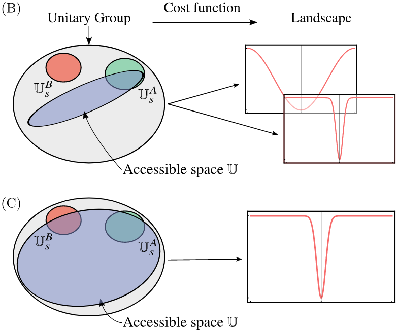
Image source: 10. A highly expressive ansatz that can access much of the space of possible unitaries (i.e., an ansatz capable of producing unitaries in something close to a Haar-random manner) is very likely to have flat cost landscapes and suffer from the barren plateau problem.

It turns out that the types of ansaetze know as hardware-efficient ansaetze also suffer from this problem if they are “random enough” (this notion will be formalized in a future demo). It was shown in 9 that this is a consequence of the concentration of measure phenomenon described above. The values of gradients and variances can be computed for classes of circuits on average by integrating with respect to the Haar measure, and it is shown that these values decrease exponentially in the number of qubits, and thus huge swaths of the cost landscape are simply and fundamentally flat.

Conclusion

The Haar measure plays an important role in quantum computing—anywhere you might be dealing with sampling random circuits, or averaging over all possible unitary operations, you’ll want to do so with respect to the Haar measure.

There are two important aspects of this that we have yet to touch upon, however. The first is whether it is efficient to sample from the Haar measure—given that the number of parameters to keep track of is exponential in the number of qubits, certainly not. But a more interesting question is do we need to always sample from the full Haar measure? The answer to this is “no” in a very interesting way. Depending on the task at hand, you may be able to take a shortcut using something called a unitary design. In an upcoming demo, we will explore the amazing world of unitary designs and their applications!

References

1

M. A. Nielsen, and I. L. Chuang (2000) “Quantum Computation and Quantum Information”, Cambridge University Press.

2(1,2,3)

H. de Guise, O. Di Matteo, and L. L. Sánchez-Soto. (2018) “Simple factorization of unitary transformations”, Phys. Rev. A 97 022328. (arXiv)

3

W. R. Clements, P. C. Humphreys, B. J. Metcalf, W. S. Kolthammer, and I. A. Walmsley (2016) “Optimal design for universal multiport interferometers”, Optica 3, 1460–1465. (arXiv)

4

M. Reck, A. Zeilinger, H. J. Bernstein, and P. Bertani (1994) “Experimental realization of any discrete unitary operator”, Phys. Rev. Lett.73, 58–61.

5(1,2,3)

F. Mezzadri (2006) “How to generate random matrices from the classical compact groups”. (arXiv)

6

E. Meckes (2019) “The Random Matrix Theory of the Classical Compact Groups”, Cambridge University Press.

7

M. Gerken (2013) “Measure concentration: Levy’s Lemma” (lecture notes).

8(1,2)

P. Hayden, D. W. Leung, and A. Winter (2006) “Aspects of generic entanglement”, Comm. Math. Phys. Vol. 265, No. 1, pp. 95-117. (arXiv)

9(1,2)

J. R. McClean, S. Boixo, V. N. Smelyanskiy, R. Babbush, and H. Neven (2018) “Barren plateaus in quantum neural network training landscapes”, Nature Communications, 9(1). (arXiv)

10(1,2,3)

Z. Holmes, K. Sharma, M. Cerezo, and P. J. Coles (2021) “Connecting ansatz expressibility to gradient magnitudes and barren plateaus”. (arXiv)

About the author

Olivia Di Matteo

Olivia is an Assistant Professor in the Department of Electrical and Computer Engineering at The University of British Columbia. Her research interests are quantum compilation, software, and algorithms.

demos/tutorial_haar_measure

 

Download Python script

 

Download Notebook

 

View on GitHub