Quantum generative adversarial networks with Cirq + TensorFlow

Author: Nathan Killoran — Posted: 11 October 2019. Last updated: 30 January 2023.

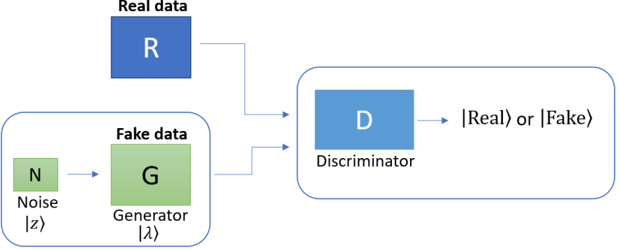
This demo constructs a Quantum Generative Adversarial Network (QGAN) (Lloyd and Weedbrook (2018), Dallaire-Demers and Killoran (2018)) using two subcircuits, a generator and a discriminator. The generator attempts to generate synthetic quantum data to match a pattern of “real” data, while the discriminator tries to discern real data from fake data (see image below). The gradient of the discriminator’s output provides a training signal for the generator to improve its fake generated data.

Using Cirq + TensorFlow

PennyLane allows us to mix and match quantum devices and classical machine learning software. For this demo, we will link together Google’s Cirq and TensorFlow libraries.

We begin by importing PennyLane, NumPy, and TensorFlow.

import numpy as np
import pennylane as qml
import tensorflow as tf

We also declare a 3-qubit simulator device running in Cirq.

dev = qml.device('cirq.simulator', wires=3)

Generator and Discriminator

In classical GANs, the starting point is to draw samples either from some “real data” distribution, or from the generator, and feed them to the discriminator. In this QGAN example, we will use a quantum circuit to generate the real data.

For this simple example, our real data will be a qubit that has been rotated (from the starting state \(\left|0\right\rangle\)) to some arbitrary, but fixed, state.

def real(angles, **kwargs):
    qml.Hadamard(wires=0)
    qml.Rot(*angles, wires=0)

For the generator and discriminator, we will choose the same basic circuit structure, but acting on different wires.

Both the real data circuit and the generator will output on wire 0, which will be connected as an input to the discriminator. Wire 1 is provided as a workspace for the generator, while the discriminator’s output will be on wire 2.

def generator(w, **kwargs):
    qml.Hadamard(wires=0)
    qml.RX(w[0], wires=0)
    qml.RX(w[1], wires=1)
    qml.RY(w[2], wires=0)
    qml.RY(w[3], wires=1)
    qml.RZ(w[4], wires=0)
    qml.RZ(w[5], wires=1)
    qml.CNOT(wires=[0, 1])
    qml.RX(w[6], wires=0)
    qml.RY(w[7], wires=0)
    qml.RZ(w[8], wires=0)


def discriminator(w):
    qml.Hadamard(wires=0)
    qml.RX(w[0], wires=0)
    qml.RX(w[1], wires=2)
    qml.RY(w[2], wires=0)
    qml.RY(w[3], wires=2)
    qml.RZ(w[4], wires=0)
    qml.RZ(w[5], wires=2)
    qml.CNOT(wires=[0, 2])
    qml.RX(w[6], wires=2)
    qml.RY(w[7], wires=2)
    qml.RZ(w[8], wires=2)

We create two QNodes. One where the real data source is wired up to the discriminator, and one where the generator is connected to the discriminator. In order to pass TensorFlow Variables into the quantum circuits, we specify the "tf" interface.

@qml.qnode(dev, interface="tf")
def real_disc_circuit(phi, theta, omega, disc_weights):
    real([phi, theta, omega])
    discriminator(disc_weights)
    return qml.expval(qml.PauliZ(2))


@qml.qnode(dev, interface="tf")
def gen_disc_circuit(gen_weights, disc_weights):
    generator(gen_weights)
    discriminator(disc_weights)
    return qml.expval(qml.PauliZ(2))

QGAN cost functions

There are two cost functions of interest, corresponding to the two stages of QGAN training. These cost functions are built from two pieces: the first piece is the probability that the discriminator correctly classifies real data as real. The second piece is the probability that the discriminator classifies fake data (i.e., a state prepared by the generator) as real.

The discriminator is trained to maximize the probability of correctly classifying real data, while minimizing the probability of mistakenly classifying fake data.

\[Cost_D = \mathrm{Pr}(real|\mathrm{fake}) - \mathrm{Pr}(real|\mathrm{real})\]

The generator is trained to maximize the probability that the discriminator accepts fake data as real.

\[Cost_G = - \mathrm{Pr}(real|\mathrm{fake})\]

def prob_real_true(disc_weights):
    true_disc_output = real_disc_circuit(phi, theta, omega, disc_weights)
    # convert to probability
    prob_real_true = (true_disc_output + 1) / 2
    return prob_real_true


def prob_fake_true(gen_weights, disc_weights):
    fake_disc_output = gen_disc_circuit(gen_weights, disc_weights)
    # convert to probability
    prob_fake_true = (fake_disc_output + 1) / 2
    return prob_fake_true


def disc_cost(disc_weights):
    cost = prob_fake_true(gen_weights, disc_weights) - prob_real_true(disc_weights)
    return cost


def gen_cost(gen_weights):
    return -prob_fake_true(gen_weights, disc_weights)

Training the QGAN

We initialize the fixed angles of the “real data” circuit, as well as the initial parameters for both generator and discriminator. These are chosen so that the generator initially prepares a state on wire 0 that is very close to the \(\left| 1 \right\rangle\) state.

phi = np.pi / 6
theta = np.pi / 2
omega = np.pi / 7
np.random.seed(0)
eps = 1e-2
init_gen_weights = np.array([np.pi] + [0] * 8) + \
                   np.random.normal(scale=eps, size=(9,))
init_disc_weights = np.random.normal(size=(9,))

gen_weights = tf.Variable(init_gen_weights)
disc_weights = tf.Variable(init_disc_weights)

We begin by creating the optimizer:

opt = tf.keras.optimizers.SGD(0.4)

In the first stage of training, we optimize the discriminator while keeping the generator parameters fixed.

cost = lambda: disc_cost(disc_weights)

for step in range(50):
    opt.minimize(cost, disc_weights)
    if step % 5 == 0:
        cost_val = cost().numpy()
        print("Step {}: cost = {}".format(step, cost_val))

Out:

Step 0: cost = -0.057276904582977295
Step 5: cost = -0.2634810581803322
Step 10: cost = -0.42739149928092957
Step 15: cost = -0.4726157709956169
Step 20: cost = -0.48406896740198135
Step 25: cost = -0.4894639253616333
Step 30: cost = -0.4928186237812042
Step 35: cost = -0.4949491620063782
Step 40: cost = -0.4962702840566635
Step 45: cost = -0.4970718026161194

At the discriminator’s optimum, the probability for the discriminator to correctly classify the real data should be close to one.

print("Prob(real classified as real): ", prob_real_true(disc_weights).numpy())

Out:

Prob(real classified as real):  0.9985870718955994

For comparison, we check how the discriminator classifies the generator’s (still unoptimized) fake data:

print("Prob(fake classified as real): ", prob_fake_true(gen_weights, disc_weights).numpy())

Out:

Prob(fake classified as real):  0.5011128038167953

In the adversarial game we now have to train the generator to better fool the discriminator. For this demo, we only perform one stage of the game. For more complex models, we would continue training the models in an alternating fashion until we reach the optimum point of the two-player adversarial game.

cost = lambda: gen_cost(gen_weights)

for step in range(50):
    opt.minimize(cost, gen_weights)
    if step % 5 == 0:
        cost_val = cost().numpy()
        print("Step {}: cost = {}".format(step, cost_val))

Out:

Step 0: cost = -0.5833386406302452
Step 5: cost = -0.8915732204914093
Step 10: cost = -0.9784242212772369
Step 15: cost = -0.9946482181549072
Step 20: cost = -0.9984995126724243
Step 25: cost = -0.9995637834072113
Step 30: cost = -0.9998717606067657
Step 35: cost = -0.999961793422699
Step 40: cost = -0.9999887347221375
Step 45: cost = -0.9999964535236359

At the optimum of the generator, the probability for the discriminator to be fooled should be close to 1.

print("Prob(fake classified as real): ", prob_fake_true(gen_weights, disc_weights).numpy())

Out:

Prob(fake classified as real):  0.9999987185001373

At the joint optimum the discriminator cost will be close to zero, indicating that the discriminator assigns equal probability to both real and generated data.

print("Discriminator cost: ", disc_cost(disc_weights).numpy())

Out:

Discriminator cost:  0.0014116466045379639

The generator has successfully learned how to simulate the real data enough to fool the discriminator.

Let’s conclude by comparing the states of the real data circuit and the generator. We expect the generator to have learned to be in a state that is very close to the one prepared in the real data circuit. An easy way to access the state of the first qubit is through its Bloch sphere representation:

obs = [qml.PauliX(0), qml.PauliY(0), qml.PauliZ(0)]

@qml.qnode(dev, interface="tf")
def bloch_vector_real(angles):
    real(angles)
    return [qml.expval(o) for o in obs]

@qml.qnode(dev, interface="tf")
def bloch_vector_generator(angles):
    generator(angles)
    return [qml.expval(o) for o in obs]

print(f"Real Bloch vector: {bloch_vector_real([phi, theta, omega])}")
print(f"Generator Bloch vector: {bloch_vector_generator(gen_weights)}")

Out:

Real Bloch vector: [<tf.Tensor: shape=(), dtype=float64, numpy=-0.21694186329841614>, <tf.Tensor: shape=(), dtype=float64, numpy=0.45048439502716064>, <tf.Tensor: shape=(), dtype=float64, numpy=-0.8660252690315247>]
Generator Bloch vector: [<tf.Tensor: shape=(), dtype=float64, numpy=-0.28404659032821655>, <tf.Tensor: shape=(), dtype=float64, numpy=0.4189322590827942>, <tf.Tensor: shape=(), dtype=float64, numpy=-0.8624440431594849>]

About the author

Nathan Killoran

Nathan is the Chief Technical Officer—Software at Xanadu. You might recognize him from his work on PennyLane, quantum machine learning, and founding the famous QHack Meme Contest.

demos/tutorial_QGAN

 

Download Python script

 

Download Notebook

 

View on GitHub