Quantum transfer learning

Author: Andrea Mari — Posted: 19 December 2019. Last updated: 28 January 2021.

In this tutorial we apply a machine learning method, known as transfer learning, to an image classifier based on a hybrid classical-quantum network.

This example follows the general structure of the PyTorch tutorial on transfer learning by Sasank Chilamkurthy, with the crucial difference of using a quantum circuit to perform the final classification task.

More details on this topic can be found in the research paper [1] (Mari et al. (2019)).

Introduction

Transfer learning is a well-established technique for training artificial neural networks (see e.g., Ref. [2]), which is based on the general intuition that if a pre-trained network is good at solving a given problem, then, with just a bit of additional training, it can be used to also solve a different but related problem.

As discussed in Ref. [1], this idea can be formalized in terms of two abstract networks \(A\) and \(B\), independently from their quantum or classical physical nature.

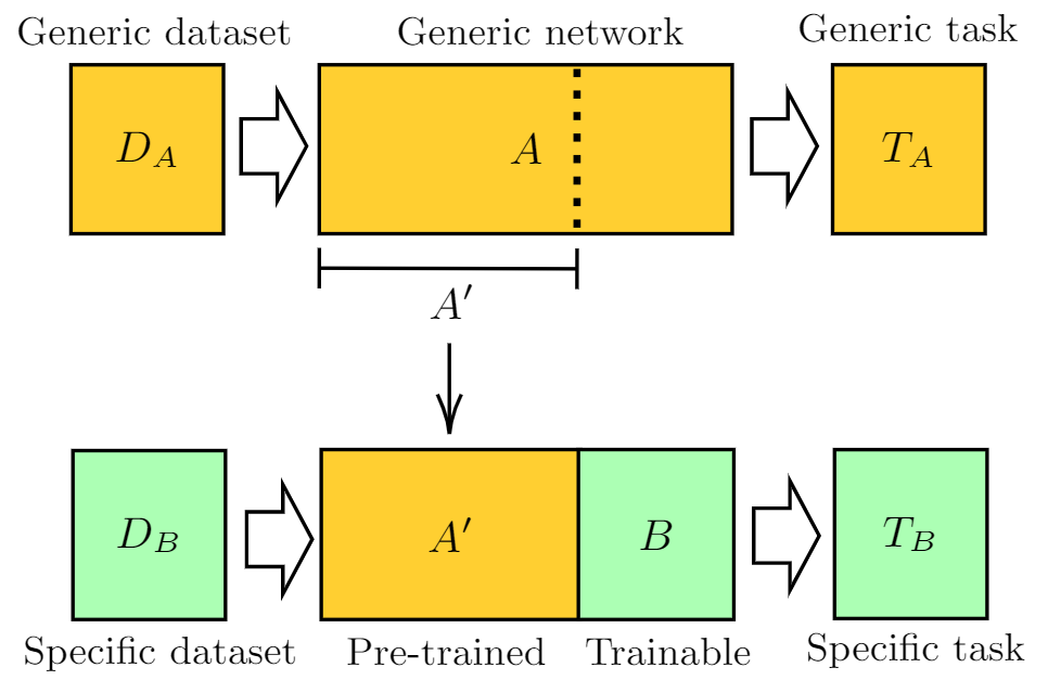
As sketched in the above figure, one can give the following general definition of the transfer learning method:

1. Take a network \(A\) that has been pre-trained on a dataset \(D_A\) and for a given task \(T_A\).

2. Remove some of the final layers. In this way, the resulting truncated network \(A'\) can be used as a feature extractor.

3. Connect a new trainable network \(B\) at the end of the pre-trained network \(A'\).

4. Keep the weights of \(A'\) constant, and train the final block \(B\) with a new dataset \(D_B\) and/or for a new task of interest \(T_B\).

When dealing with hybrid systems, depending on the physical nature (classical or quantum) of the networks \(A\) and \(B\), one can have different implementations of transfer learning as

summarized in following table:

Network A	Network B	Transfer learning scheme
Classical	Classical	CC - Standard classical method. See e.g., Ref. [2].
Classical	Quantum	CQ - Hybrid model presented in this tutorial.
Quantum	Classical	QC - Model studied in Ref. [1].
Quantum	Quantum	QQ - Model studied in Ref. [1].

Classical-to-quantum transfer learning

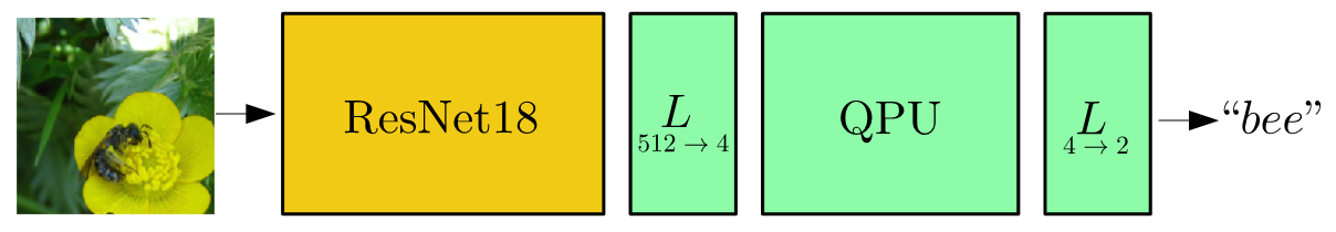
We focus on the CQ transfer learning scheme discussed in the previous section and we give a specific example.

1. As pre-trained network \(A\) we use ResNet18, a deep residual neural network introduced by Microsoft in Ref. [3], which is pre-trained on the ImageNet dataset.

2. After removing its final layer we obtain \(A'\), a pre-processing block which maps any input high-resolution image into 512 abstract features.

3. Such features are classified by a 4-qubit “dressed quantum circuit” \(B\), i.e., a variational quantum circuit sandwiched between two classical layers.

4. The hybrid model is trained, keeping \(A'\) constant, on the Hymenoptera dataset (a small subclass of ImageNet) containing images of ants and bees.

A graphical representation of the full data processing pipeline is given in the figure below.

General setup

Note

To use the PyTorch interface in PennyLane, you must first install PyTorch.

In addition to PennyLane, we will also need some standard PyTorch libraries and the plotting library matplotlib.

# Some parts of this code are based on the Python script:
# https://github.com/pytorch/tutorials/blob/master/beginner_source/transfer_learning_tutorial.py
# License: BSD

import time
import os
import copy

# PyTorch
import torch
import torch.nn as nn
import torch.optim as optim
from torch.optim import lr_scheduler
import torchvision
from torchvision import datasets, transforms

# Pennylane
import pennylane as qml
from pennylane import numpy as np

torch.manual_seed(42)
np.random.seed(42)

# Plotting
import matplotlib.pyplot as plt

# OpenMP: number of parallel threads.
os.environ["OMP_NUM_THREADS"] = "1"

Setting of the main hyper-parameters of the model

Note

To reproduce the results of Ref. [1], num_epochs should be set to 30 which may take a long time. We suggest to first try with num_epochs=1 and, if everything runs smoothly, increase it to a larger value.

n_qubits = 4                # Number of qubits
step = 0.0004               # Learning rate
batch_size = 4              # Number of samples for each training step
num_epochs = 3              # Number of training epochs
q_depth = 6                 # Depth of the quantum circuit (number of variational layers)
gamma_lr_scheduler = 0.1    # Learning rate reduction applied every 10 epochs.
q_delta = 0.01              # Initial spread of random quantum weights
start_time = time.time()    # Start of the computation timer

We initialize a PennyLane device with a default.qubit backend.

dev = qml.device("default.qubit", wires=n_qubits)

We configure PyTorch to use CUDA only if available. Otherwise the CPU is used.

device = torch.device("cuda:0" if torch.cuda.is_available() else "cpu")

Dataset loading

Note

The dataset containing images of ants and bees can be downloaded here and should be extracted in the subfolder ../_data/hymenoptera_data.

This is a very small dataset (roughly 250 images), too small for training from scratch a classical or quantum model, however it is enough when using transfer learning approach.

The PyTorch packages torchvision and torch.utils.data are used for loading the dataset and performing standard preliminary image operations: resize, center, crop, normalize, etc.

data_transforms = {
    "train": transforms.Compose(
        [
            # transforms.RandomResizedCrop(224),     # uncomment for data augmentation
            # transforms.RandomHorizontalFlip(),     # uncomment for data augmentation
            transforms.Resize(256),
            transforms.CenterCrop(224),
            transforms.ToTensor(),
            # Normalize input channels using mean values and standard deviations of ImageNet.
            transforms.Normalize([0.485, 0.456, 0.406], [0.229, 0.224, 0.225]),
        ]
    ),
    "val": transforms.Compose(
        [
            transforms.Resize(256),
            transforms.CenterCrop(224),
            transforms.ToTensor(),
            transforms.Normalize([0.485, 0.456, 0.406], [0.229, 0.224, 0.225]),
        ]
    ),
}

data_dir = "../_data/hymenoptera_data"
image_datasets = {
    x if x == "train" else "validation": datasets.ImageFolder(
        os.path.join(data_dir, x), data_transforms[x]
    )
    for x in ["train", "val"]
}
dataset_sizes = {x: len(image_datasets[x]) for x in ["train", "validation"]}
class_names = image_datasets["train"].classes

# Initialize dataloader
dataloaders = {
    x: torch.utils.data.DataLoader(image_datasets[x], batch_size=batch_size, shuffle=True)
    for x in ["train", "validation"]
}

# function to plot images
def imshow(inp, title=None):
    """Display image from tensor."""
    inp = inp.numpy().transpose((1, 2, 0))
    # Inverse of the initial normalization operation.
    mean = np.array([0.485, 0.456, 0.406])
    std = np.array([0.229, 0.224, 0.225])
    inp = std * inp + mean
    inp = np.clip(inp, 0, 1)
    plt.imshow(inp)
    if title is not None:
        plt.title(title)

Let us show a batch of the test data, just to have an idea of the classification problem.

# Get a batch of training data
inputs, classes = next(iter(dataloaders["validation"]))

# Make a grid from batch
out = torchvision.utils.make_grid(inputs)

imshow(out, title=[class_names[x] for x in classes])

dataloaders = {
    x: torch.utils.data.DataLoader(image_datasets[x], batch_size=batch_size, shuffle=True)
    for x in ["train", "validation"]
}

Variational quantum circuit

We first define some quantum layers that will compose the quantum circuit.

def H_layer(nqubits):
    """Layer of single-qubit Hadamard gates.
    """
    for idx in range(nqubits):
        qml.Hadamard(wires=idx)


def RY_layer(w):
    """Layer of parametrized qubit rotations around the y axis.
    """
    for idx, element in enumerate(w):
        qml.RY(element, wires=idx)


def entangling_layer(nqubits):
    """Layer of CNOTs followed by another shifted layer of CNOT.
    """
    # In other words it should apply something like :
    # CNOT  CNOT  CNOT  CNOT...  CNOT
    #   CNOT  CNOT  CNOT...  CNOT
    for i in range(0, nqubits - 1, 2):  # Loop over even indices: i=0,2,...N-2
        qml.CNOT(wires=[i, i + 1])
    for i in range(1, nqubits - 1, 2):  # Loop over odd indices:  i=1,3,...N-3
        qml.CNOT(wires=[i, i + 1])

Now we define the quantum circuit through the PennyLane qnode decorator .

The structure is that of a typical variational quantum circuit:

• Embedding layer: All qubits are first initialized in a balanced superposition of up and down states, then they are rotated according to the input parameters (local embedding).

• Variational layers: A sequence of trainable rotation layers and constant entangling layers is applied.

• Measurement layer: For each qubit, the local expectation value of the \(Z\) operator is measured. This produces a classical output vector, suitable for additional post-processing.

@qml.qnode(dev, interface="torch")
def quantum_net(q_input_features, q_weights_flat):
    """
    The variational quantum circuit.
    """

    # Reshape weights
    q_weights = q_weights_flat.reshape(q_depth, n_qubits)

    # Start from state |+> , unbiased w.r.t. |0> and |1>
    H_layer(n_qubits)

    # Embed features in the quantum node
    RY_layer(q_input_features)

    # Sequence of trainable variational layers
    for k in range(q_depth):
        entangling_layer(n_qubits)
        RY_layer(q_weights[k])

    # Expectation values in the Z basis
    exp_vals = [qml.expval(qml.PauliZ(position)) for position in range(n_qubits)]
    return tuple(exp_vals)

Dressed quantum circuit

We can now define a custom torch.nn.Module representing a dressed quantum circuit.

This is a concatenation of:

• A classical pre-processing layer (nn.Linear).

• A classical activation function (torch.tanh).

• A constant np.pi/2.0 scaling.

• The previously defined quantum circuit (quantum_net).

• A classical post-processing layer (nn.Linear).

The input of the module is a batch of vectors with 512 real parameters (features) and the output is a batch of vectors with two real outputs (associated with the two classes of images: ants and bees).

class DressedQuantumNet(nn.Module):
    """
    Torch module implementing the *dressed* quantum net.
    """

    def __init__(self):
        """
        Definition of the *dressed* layout.
        """

        super().__init__()
        self.pre_net = nn.Linear(512, n_qubits)
        self.q_params = nn.Parameter(q_delta * torch.randn(q_depth * n_qubits))
        self.post_net = nn.Linear(n_qubits, 2)

    def forward(self, input_features):
        """
        Defining how tensors are supposed to move through the *dressed* quantum
        net.
        """

        # obtain the input features for the quantum circuit
        # by reducing the feature dimension from 512 to 4
        pre_out = self.pre_net(input_features)
        q_in = torch.tanh(pre_out) * np.pi / 2.0

        # Apply the quantum circuit to each element of the batch and append to q_out
        q_out = torch.Tensor(0, n_qubits)
        q_out = q_out.to(device)
        for elem in q_in:
            q_out_elem = torch.hstack(quantum_net(elem, self.q_params)).float().unsqueeze(0)
            q_out = torch.cat((q_out, q_out_elem))

        # return the two-dimensional prediction from the postprocessing layer
        return self.post_net(q_out)

Hybrid classical-quantum model

We are finally ready to build our full hybrid classical-quantum network. We follow the transfer learning approach:

1. First load the classical pre-trained network ResNet18 from the torchvision.models zoo.

2. Freeze all the weights since they should not be trained.

3. Replace the last fully connected layer with our trainable dressed quantum circuit (DressedQuantumNet).

Note

The ResNet18 model is automatically downloaded by PyTorch and it may take several minutes (only the first time).

model_hybrid = torchvision.models.resnet18(pretrained=True)

for param in model_hybrid.parameters():
    param.requires_grad = False


# Notice that model_hybrid.fc is the last layer of ResNet18
model_hybrid.fc = DressedQuantumNet()

# Use CUDA or CPU according to the "device" object.
model_hybrid = model_hybrid.to(device)

Out:

Downloading: "https://download.pytorch.org/models/resnet18-f37072fd.pth" to /home/runner/.cache/torch/hub/checkpoints/resnet18-f37072fd.pth

  0%|          | 0.00/44.7M [00:00<?, ?B/s]
 58%|#####7    | 25.9M/44.7M [00:00<00:00, 271MB/s]
100%|##########| 44.7M/44.7M [00:00<00:00, 277MB/s]

Training and results

Before training the network we need to specify the loss function.

We use, as usual in classification problem, the cross-entropy which is directly available within torch.nn.

criterion = nn.CrossEntropyLoss()

We also initialize the Adam optimizer which is called at each training step in order to update the weights of the model.

optimizer_hybrid = optim.Adam(model_hybrid.fc.parameters(), lr=step)

We schedule to reduce the learning rate by a factor of gamma_lr_scheduler every 10 epochs.

exp_lr_scheduler = lr_scheduler.StepLR(
    optimizer_hybrid, step_size=10, gamma=gamma_lr_scheduler
)

What follows is a training function that will be called later. This function should return a trained model that can be used to make predictions (classifications).

def train_model(model, criterion, optimizer, scheduler, num_epochs):
    since = time.time()
    best_model_wts = copy.deepcopy(model.state_dict())
    best_acc = 0.0
    best_loss = 10000.0  # Large arbitrary number
    best_acc_train = 0.0
    best_loss_train = 10000.0  # Large arbitrary number
    print("Training started:")

    for epoch in range(num_epochs):

        # Each epoch has a training and validation phase
        for phase in ["train", "validation"]:
            if phase == "train":
                # Set model to training mode
                model.train()
            else:
                # Set model to evaluate mode
                model.eval()
            running_loss = 0.0
            running_corrects = 0

            # Iterate over data.
            n_batches = dataset_sizes[phase] // batch_size
            it = 0
            for inputs, labels in dataloaders[phase]:
                since_batch = time.time()
                batch_size_ = len(inputs)
                inputs = inputs.to(device)
                labels = labels.to(device)
                optimizer.zero_grad()

                # Track/compute gradient and make an optimization step only when training
                with torch.set_grad_enabled(phase == "train"):
                    outputs = model(inputs)
                    _, preds = torch.max(outputs, 1)
                    loss = criterion(outputs, labels)
                    if phase == "train":
                        loss.backward()
                        optimizer.step()

                # Print iteration results
                running_loss += loss.item() * batch_size_
                batch_corrects = torch.sum(preds == labels.data).item()
                running_corrects += batch_corrects
                print(
                    "Phase: {} Epoch: {}/{} Iter: {}/{} Batch time: {:.4f}".format(
                        phase,
                        epoch + 1,
                        num_epochs,
                        it + 1,
                        n_batches + 1,
                        time.time() - since_batch,
                    ),
                    end="\r",
                    flush=True,
                )
                it += 1

            # Print epoch results
            epoch_loss = running_loss / dataset_sizes[phase]
            epoch_acc = running_corrects / dataset_sizes[phase]
            print(
                "Phase: {} Epoch: {}/{} Loss: {:.4f} Acc: {:.4f}        ".format(
                    "train" if phase == "train" else "validation  ",
                    epoch + 1,
                    num_epochs,
                    epoch_loss,
                    epoch_acc,
                )
            )

            # Check if this is the best model wrt previous epochs
            if phase == "validation" and epoch_acc > best_acc:
                best_acc = epoch_acc
                best_model_wts = copy.deepcopy(model.state_dict())
            if phase == "validation" and epoch_loss < best_loss:
                best_loss = epoch_loss
            if phase == "train" and epoch_acc > best_acc_train:
                best_acc_train = epoch_acc
            if phase == "train" and epoch_loss < best_loss_train:
                best_loss_train = epoch_loss

            # Update learning rate
            if phase == "train":
                scheduler.step()

    # Print final results
    model.load_state_dict(best_model_wts)
    time_elapsed = time.time() - since
    print(
        "Training completed in {:.0f}m {:.0f}s".format(time_elapsed // 60, time_elapsed % 60)
    )
    print("Best test loss: {:.4f} | Best test accuracy: {:.4f}".format(best_loss, best_acc))
    return model

We are ready to perform the actual training process.

model_hybrid = train_model(
    model_hybrid, criterion, optimizer_hybrid, exp_lr_scheduler, num_epochs=num_epochs
)

Out:

Training started:
Phase: train Epoch: 1/3 Iter: 1/62 Batch time: 0.2366
Phase: train Epoch: 1/3 Iter: 2/62 Batch time: 0.2234
Phase: train Epoch: 1/3 Iter: 3/62 Batch time: 0.2116
Phase: train Epoch: 1/3 Iter: 4/62 Batch time: 0.2245
Phase: train Epoch: 1/3 Iter: 5/62 Batch time: 0.2174
Phase: train Epoch: 1/3 Iter: 6/62 Batch time: 0.2184
Phase: train Epoch: 1/3 Iter: 7/62 Batch time: 0.2157
Phase: train Epoch: 1/3 Iter: 8/62 Batch time: 0.2182
Phase: train Epoch: 1/3 Iter: 9/62 Batch time: 0.2168
Phase: train Epoch: 1/3 Iter: 10/62 Batch time: 0.2151
Phase: train Epoch: 1/3 Iter: 11/62 Batch time: 0.2151
Phase: train Epoch: 1/3 Iter: 12/62 Batch time: 0.2173
Phase: train Epoch: 1/3 Iter: 13/62 Batch time: 0.2191
Phase: train Epoch: 1/3 Iter: 14/62 Batch time: 0.2167
Phase: train Epoch: 1/3 Iter: 15/62 Batch time: 0.2188
Phase: train Epoch: 1/3 Iter: 16/62 Batch time: 0.2158
Phase: train Epoch: 1/3 Iter: 17/62 Batch time: 0.2145
Phase: train Epoch: 1/3 Iter: 18/62 Batch time: 0.2148
Phase: train Epoch: 1/3 Iter: 19/62 Batch time: 0.2141
Phase: train Epoch: 1/3 Iter: 20/62 Batch time: 0.2153
Phase: train Epoch: 1/3 Iter: 21/62 Batch time: 0.2175
Phase: train Epoch: 1/3 Iter: 22/62 Batch time: 0.2166
Phase: train Epoch: 1/3 Iter: 23/62 Batch time: 0.2176
Phase: train Epoch: 1/3 Iter: 24/62 Batch time: 0.2159
Phase: train Epoch: 1/3 Iter: 25/62 Batch time: 0.2163
Phase: train Epoch: 1/3 Iter: 26/62 Batch time: 0.2170
Phase: train Epoch: 1/3 Iter: 27/62 Batch time: 0.2196
Phase: train Epoch: 1/3 Iter: 28/62 Batch time: 0.2185
Phase: train Epoch: 1/3 Iter: 29/62 Batch time: 0.2183
Phase: train Epoch: 1/3 Iter: 30/62 Batch time: 0.2182
Phase: train Epoch: 1/3 Iter: 31/62 Batch time: 0.2258
Phase: train Epoch: 1/3 Iter: 32/62 Batch time: 0.2188
Phase: train Epoch: 1/3 Iter: 33/62 Batch time: 0.2187
Phase: train Epoch: 1/3 Iter: 34/62 Batch time: 0.2151
Phase: train Epoch: 1/3 Iter: 35/62 Batch time: 0.2177
Phase: train Epoch: 1/3 Iter: 36/62 Batch time: 0.2174
Phase: train Epoch: 1/3 Iter: 37/62 Batch time: 0.2208
Phase: train Epoch: 1/3 Iter: 38/62 Batch time: 0.2206
Phase: train Epoch: 1/3 Iter: 39/62 Batch time: 0.2180
Phase: train Epoch: 1/3 Iter: 40/62 Batch time: 0.2169
Phase: train Epoch: 1/3 Iter: 41/62 Batch time: 0.2190
Phase: train Epoch: 1/3 Iter: 42/62 Batch time: 0.2170
Phase: train Epoch: 1/3 Iter: 43/62 Batch time: 0.2185
Phase: train Epoch: 1/3 Iter: 44/62 Batch time: 0.2162
Phase: train Epoch: 1/3 Iter: 45/62 Batch time: 0.2188
Phase: train Epoch: 1/3 Iter: 46/62 Batch time: 0.2172
Phase: train Epoch: 1/3 Iter: 47/62 Batch time: 0.2170
Phase: train Epoch: 1/3 Iter: 48/62 Batch time: 0.2209
Phase: train Epoch: 1/3 Iter: 49/62 Batch time: 0.2204
Phase: train Epoch: 1/3 Iter: 50/62 Batch time: 0.2219
Phase: train Epoch: 1/3 Iter: 51/62 Batch time: 0.2149
Phase: train Epoch: 1/3 Iter: 52/62 Batch time: 0.2208
Phase: train Epoch: 1/3 Iter: 53/62 Batch time: 0.2187
Phase: train Epoch: 1/3 Iter: 54/62 Batch time: 0.2194
Phase: train Epoch: 1/3 Iter: 55/62 Batch time: 0.2179
Phase: train Epoch: 1/3 Iter: 56/62 Batch time: 0.2178
Phase: train Epoch: 1/3 Iter: 57/62 Batch time: 0.2209
Phase: train Epoch: 1/3 Iter: 58/62 Batch time: 0.2192
Phase: train Epoch: 1/3 Iter: 59/62 Batch time: 0.2197
Phase: train Epoch: 1/3 Iter: 60/62 Batch time: 0.2183
Phase: train Epoch: 1/3 Iter: 61/62 Batch time: 0.2220
Phase: train Epoch: 1/3 Loss: 0.6990 Acc: 0.5246
Phase: validation Epoch: 1/3 Iter: 1/39 Batch time: 0.1621
Phase: validation Epoch: 1/3 Iter: 2/39 Batch time: 0.1595
Phase: validation Epoch: 1/3 Iter: 3/39 Batch time: 0.1592
Phase: validation Epoch: 1/3 Iter: 4/39 Batch time: 0.1586
Phase: validation Epoch: 1/3 Iter: 5/39 Batch time: 0.1584
Phase: validation Epoch: 1/3 Iter: 6/39 Batch time: 0.1602
Phase: validation Epoch: 1/3 Iter: 7/39 Batch time: 0.1585
Phase: validation Epoch: 1/3 Iter: 8/39 Batch time: 0.1561
Phase: validation Epoch: 1/3 Iter: 9/39 Batch time: 0.1554
Phase: validation Epoch: 1/3 Iter: 10/39 Batch time: 0.1586
Phase: validation Epoch: 1/3 Iter: 11/39 Batch time: 0.1586
Phase: validation Epoch: 1/3 Iter: 12/39 Batch time: 0.1587
Phase: validation Epoch: 1/3 Iter: 13/39 Batch time: 0.1577
Phase: validation Epoch: 1/3 Iter: 14/39 Batch time: 0.1555
Phase: validation Epoch: 1/3 Iter: 15/39 Batch time: 0.1580
Phase: validation Epoch: 1/3 Iter: 16/39 Batch time: 0.1588
Phase: validation Epoch: 1/3 Iter: 17/39 Batch time: 0.1622
Phase: validation Epoch: 1/3 Iter: 18/39 Batch time: 0.1586
Phase: validation Epoch: 1/3 Iter: 19/39 Batch time: 0.1557
Phase: validation Epoch: 1/3 Iter: 20/39 Batch time: 0.1589
Phase: validation Epoch: 1/3 Iter: 21/39 Batch time: 0.1598
Phase: validation Epoch: 1/3 Iter: 22/39 Batch time: 0.1583
Phase: validation Epoch: 1/3 Iter: 23/39 Batch time: 0.1570
Phase: validation Epoch: 1/3 Iter: 24/39 Batch time: 0.1567
Phase: validation Epoch: 1/3 Iter: 25/39 Batch time: 0.1554
Phase: validation Epoch: 1/3 Iter: 26/39 Batch time: 0.1587
Phase: validation Epoch: 1/3 Iter: 27/39 Batch time: 0.1564
Phase: validation Epoch: 1/3 Iter: 28/39 Batch time: 0.1573
Phase: validation Epoch: 1/3 Iter: 29/39 Batch time: 0.1587
Phase: validation Epoch: 1/3 Iter: 30/39 Batch time: 0.1584
Phase: validation Epoch: 1/3 Iter: 31/39 Batch time: 0.1575
Phase: validation Epoch: 1/3 Iter: 32/39 Batch time: 0.1582
Phase: validation Epoch: 1/3 Iter: 33/39 Batch time: 0.1592
Phase: validation Epoch: 1/3 Iter: 34/39 Batch time: 0.1561
Phase: validation Epoch: 1/3 Iter: 35/39 Batch time: 0.1552
Phase: validation Epoch: 1/3 Iter: 36/39 Batch time: 0.1543
Phase: validation Epoch: 1/3 Iter: 37/39 Batch time: 0.1561
Phase: validation Epoch: 1/3 Iter: 38/39 Batch time: 0.1551
Phase: validation Epoch: 1/3 Iter: 39/39 Batch time: 0.0506
Phase: validation   Epoch: 1/3 Loss: 0.6429 Acc: 0.6536
Phase: train Epoch: 2/3 Iter: 1/62 Batch time: 0.2089
Phase: train Epoch: 2/3 Iter: 2/62 Batch time: 0.2154
Phase: train Epoch: 2/3 Iter: 3/62 Batch time: 0.2169
Phase: train Epoch: 2/3 Iter: 4/62 Batch time: 0.2190
Phase: train Epoch: 2/3 Iter: 5/62 Batch time: 0.2157
Phase: train Epoch: 2/3 Iter: 6/62 Batch time: 0.2140
Phase: train Epoch: 2/3 Iter: 7/62 Batch time: 0.2177
Phase: train Epoch: 2/3 Iter: 8/62 Batch time: 0.2158
Phase: train Epoch: 2/3 Iter: 9/62 Batch time: 0.2176
Phase: train Epoch: 2/3 Iter: 10/62 Batch time: 0.2161
Phase: train Epoch: 2/3 Iter: 11/62 Batch time: 0.2163
Phase: train Epoch: 2/3 Iter: 12/62 Batch time: 0.2193
Phase: train Epoch: 2/3 Iter: 13/62 Batch time: 0.2187
Phase: train Epoch: 2/3 Iter: 14/62 Batch time: 0.2189
Phase: train Epoch: 2/3 Iter: 15/62 Batch time: 0.2191
Phase: train Epoch: 2/3 Iter: 16/62 Batch time: 0.2193
Phase: train Epoch: 2/3 Iter: 17/62 Batch time: 0.2183
Phase: train Epoch: 2/3 Iter: 18/62 Batch time: 0.2167
Phase: train Epoch: 2/3 Iter: 19/62 Batch time: 0.2188
Phase: train Epoch: 2/3 Iter: 20/62 Batch time: 0.2178
Phase: train Epoch: 2/3 Iter: 21/62 Batch time: 0.2311
Phase: train Epoch: 2/3 Iter: 22/62 Batch time: 0.2217
Phase: train Epoch: 2/3 Iter: 23/62 Batch time: 0.2157
Phase: train Epoch: 2/3 Iter: 24/62 Batch time: 0.2194
Phase: train Epoch: 2/3 Iter: 25/62 Batch time: 0.2272
Phase: train Epoch: 2/3 Iter: 26/62 Batch time: 0.2158
Phase: train Epoch: 2/3 Iter: 27/62 Batch time: 0.2194
Phase: train Epoch: 2/3 Iter: 28/62 Batch time: 0.2193
Phase: train Epoch: 2/3 Iter: 29/62 Batch time: 0.2180
Phase: train Epoch: 2/3 Iter: 30/62 Batch time: 0.2203
Phase: train Epoch: 2/3 Iter: 31/62 Batch time: 0.2203
Phase: train Epoch: 2/3 Iter: 32/62 Batch time: 0.2219
Phase: train Epoch: 2/3 Iter: 33/62 Batch time: 0.2215
Phase: train Epoch: 2/3 Iter: 34/62 Batch time: 0.2168
Phase: train Epoch: 2/3 Iter: 35/62 Batch time: 0.2205
Phase: train Epoch: 2/3 Iter: 36/62 Batch time: 0.2171
Phase: train Epoch: 2/3 Iter: 37/62 Batch time: 0.2206
Phase: train Epoch: 2/3 Iter: 38/62 Batch time: 0.2216
Phase: train Epoch: 2/3 Iter: 39/62 Batch time: 0.2225
Phase: train Epoch: 2/3 Iter: 40/62 Batch time: 0.2216
Phase: train Epoch: 2/3 Iter: 41/62 Batch time: 0.2183
Phase: train Epoch: 2/3 Iter: 42/62 Batch time: 0.2166
Phase: train Epoch: 2/3 Iter: 43/62 Batch time: 0.2150
Phase: train Epoch: 2/3 Iter: 44/62 Batch time: 0.2111
Phase: train Epoch: 2/3 Iter: 45/62 Batch time: 0.2117
Phase: train Epoch: 2/3 Iter: 46/62 Batch time: 0.2150
Phase: train Epoch: 2/3 Iter: 47/62 Batch time: 0.2125
Phase: train Epoch: 2/3 Iter: 48/62 Batch time: 0.2171
Phase: train Epoch: 2/3 Iter: 49/62 Batch time: 0.2146
Phase: train Epoch: 2/3 Iter: 50/62 Batch time: 0.2175
Phase: train Epoch: 2/3 Iter: 51/62 Batch time: 0.2146
Phase: train Epoch: 2/3 Iter: 52/62 Batch time: 0.2147
Phase: train Epoch: 2/3 Iter: 53/62 Batch time: 0.2159
Phase: train Epoch: 2/3 Iter: 54/62 Batch time: 0.2168
Phase: train Epoch: 2/3 Iter: 55/62 Batch time: 0.2172
Phase: train Epoch: 2/3 Iter: 56/62 Batch time: 0.2180
Phase: train Epoch: 2/3 Iter: 57/62 Batch time: 0.2169
Phase: train Epoch: 2/3 Iter: 58/62 Batch time: 0.2146
Phase: train Epoch: 2/3 Iter: 59/62 Batch time: 0.2124
Phase: train Epoch: 2/3 Iter: 60/62 Batch time: 0.2133
Phase: train Epoch: 2/3 Iter: 61/62 Batch time: 0.2170
Phase: train Epoch: 2/3 Loss: 0.6134 Acc: 0.7008
Phase: validation Epoch: 2/3 Iter: 1/39 Batch time: 0.1633
Phase: validation Epoch: 2/3 Iter: 2/39 Batch time: 0.1644
Phase: validation Epoch: 2/3 Iter: 3/39 Batch time: 0.1561
Phase: validation Epoch: 2/3 Iter: 4/39 Batch time: 0.1537
Phase: validation Epoch: 2/3 Iter: 5/39 Batch time: 0.1550
Phase: validation Epoch: 2/3 Iter: 6/39 Batch time: 0.1554
Phase: validation Epoch: 2/3 Iter: 7/39 Batch time: 0.1577
Phase: validation Epoch: 2/3 Iter: 8/39 Batch time: 0.1562
Phase: validation Epoch: 2/3 Iter: 9/39 Batch time: 0.1583
Phase: validation Epoch: 2/3 Iter: 10/39 Batch time: 0.1573
Phase: validation Epoch: 2/3 Iter: 11/39 Batch time: 0.1588
Phase: validation Epoch: 2/3 Iter: 12/39 Batch time: 0.1594
Phase: validation Epoch: 2/3 Iter: 13/39 Batch time: 0.1570
Phase: validation Epoch: 2/3 Iter: 14/39 Batch time: 0.1579
Phase: validation Epoch: 2/3 Iter: 15/39 Batch time: 0.1606
Phase: validation Epoch: 2/3 Iter: 16/39 Batch time: 0.1599
Phase: validation Epoch: 2/3 Iter: 17/39 Batch time: 0.1590
Phase: validation Epoch: 2/3 Iter: 18/39 Batch time: 0.1610
Phase: validation Epoch: 2/3 Iter: 19/39 Batch time: 0.1594
Phase: validation Epoch: 2/3 Iter: 20/39 Batch time: 0.1588
Phase: validation Epoch: 2/3 Iter: 21/39 Batch time: 0.1602
Phase: validation Epoch: 2/3 Iter: 22/39 Batch time: 0.1577
Phase: validation Epoch: 2/3 Iter: 23/39 Batch time: 0.1581
Phase: validation Epoch: 2/3 Iter: 24/39 Batch time: 0.1565
Phase: validation Epoch: 2/3 Iter: 25/39 Batch time: 0.1563
Phase: validation Epoch: 2/3 Iter: 26/39 Batch time: 0.1575
Phase: validation Epoch: 2/3 Iter: 27/39 Batch time: 0.1655
Phase: validation Epoch: 2/3 Iter: 28/39 Batch time: 0.1556
Phase: validation Epoch: 2/3 Iter: 29/39 Batch time: 0.1572
Phase: validation Epoch: 2/3 Iter: 30/39 Batch time: 0.1568
Phase: validation Epoch: 2/3 Iter: 31/39 Batch time: 0.1579
Phase: validation Epoch: 2/3 Iter: 32/39 Batch time: 0.1566
Phase: validation Epoch: 2/3 Iter: 33/39 Batch time: 0.1564
Phase: validation Epoch: 2/3 Iter: 34/39 Batch time: 0.1565
Phase: validation Epoch: 2/3 Iter: 35/39 Batch time: 0.1640
Phase: validation Epoch: 2/3 Iter: 36/39 Batch time: 0.1605
Phase: validation Epoch: 2/3 Iter: 37/39 Batch time: 0.1574
Phase: validation Epoch: 2/3 Iter: 38/39 Batch time: 0.1576
Phase: validation Epoch: 2/3 Iter: 39/39 Batch time: 0.0463
Phase: validation   Epoch: 2/3 Loss: 0.5389 Acc: 0.8235
Phase: train Epoch: 3/3 Iter: 1/62 Batch time: 0.2097
Phase: train Epoch: 3/3 Iter: 2/62 Batch time: 0.2140
Phase: train Epoch: 3/3 Iter: 3/62 Batch time: 0.2176
Phase: train Epoch: 3/3 Iter: 4/62 Batch time: 0.2158
Phase: train Epoch: 3/3 Iter: 5/62 Batch time: 0.2172
Phase: train Epoch: 3/3 Iter: 6/62 Batch time: 0.2205
Phase: train Epoch: 3/3 Iter: 7/62 Batch time: 0.2179
Phase: train Epoch: 3/3 Iter: 8/62 Batch time: 0.2181
Phase: train Epoch: 3/3 Iter: 9/62 Batch time: 0.2186
Phase: train Epoch: 3/3 Iter: 10/62 Batch time: 0.2202
Phase: train Epoch: 3/3 Iter: 11/62 Batch time: 0.2191
Phase: train Epoch: 3/3 Iter: 12/62 Batch time: 0.2172
Phase: train Epoch: 3/3 Iter: 13/62 Batch time: 0.2171
Phase: train Epoch: 3/3 Iter: 14/62 Batch time: 0.2194
Phase: train Epoch: 3/3 Iter: 15/62 Batch time: 0.2183
Phase: train Epoch: 3/3 Iter: 16/62 Batch time: 0.2195
Phase: train Epoch: 3/3 Iter: 17/62 Batch time: 0.2189
Phase: train Epoch: 3/3 Iter: 18/62 Batch time: 0.2176
Phase: train Epoch: 3/3 Iter: 19/62 Batch time: 0.2222
Phase: train Epoch: 3/3 Iter: 20/62 Batch time: 0.2233
Phase: train Epoch: 3/3 Iter: 21/62 Batch time: 0.2201
Phase: train Epoch: 3/3 Iter: 22/62 Batch time: 0.2143
Phase: train Epoch: 3/3 Iter: 23/62 Batch time: 0.2205
Phase: train Epoch: 3/3 Iter: 24/62 Batch time: 0.2158
Phase: train Epoch: 3/3 Iter: 25/62 Batch time: 0.2177
Phase: train Epoch: 3/3 Iter: 26/62 Batch time: 0.2180
Phase: train Epoch: 3/3 Iter: 27/62 Batch time: 0.2171
Phase: train Epoch: 3/3 Iter: 28/62 Batch time: 0.2164
Phase: train Epoch: 3/3 Iter: 29/62 Batch time: 0.2198
Phase: train Epoch: 3/3 Iter: 30/62 Batch time: 0.2164
Phase: train Epoch: 3/3 Iter: 31/62 Batch time: 0.2182
Phase: train Epoch: 3/3 Iter: 32/62 Batch time: 0.2272
Phase: train Epoch: 3/3 Iter: 33/62 Batch time: 0.2200
Phase: train Epoch: 3/3 Iter: 34/62 Batch time: 0.2165
Phase: train Epoch: 3/3 Iter: 35/62 Batch time: 0.2147
Phase: train Epoch: 3/3 Iter: 36/62 Batch time: 0.2151
Phase: train Epoch: 3/3 Iter: 37/62 Batch time: 0.2152
Phase: train Epoch: 3/3 Iter: 38/62 Batch time: 0.2160
Phase: train Epoch: 3/3 Iter: 39/62 Batch time: 0.2163
Phase: train Epoch: 3/3 Iter: 40/62 Batch time: 0.2162
Phase: train Epoch: 3/3 Iter: 41/62 Batch time: 0.2193
Phase: train Epoch: 3/3 Iter: 42/62 Batch time: 0.2176
Phase: train Epoch: 3/3 Iter: 43/62 Batch time: 0.2147
Phase: train Epoch: 3/3 Iter: 44/62 Batch time: 0.2169
Phase: train Epoch: 3/3 Iter: 45/62 Batch time: 0.2140
Phase: train Epoch: 3/3 Iter: 46/62 Batch time: 0.2158
Phase: train Epoch: 3/3 Iter: 47/62 Batch time: 0.2147
Phase: train Epoch: 3/3 Iter: 48/62 Batch time: 0.2239
Phase: train Epoch: 3/3 Iter: 49/62 Batch time: 0.2176
Phase: train Epoch: 3/3 Iter: 50/62 Batch time: 0.2162
Phase: train Epoch: 3/3 Iter: 51/62 Batch time: 0.2151
Phase: train Epoch: 3/3 Iter: 52/62 Batch time: 0.2142
Phase: train Epoch: 3/3 Iter: 53/62 Batch time: 0.2180
Phase: train Epoch: 3/3 Iter: 54/62 Batch time: 0.2146
Phase: train Epoch: 3/3 Iter: 55/62 Batch time: 0.2168
Phase: train Epoch: 3/3 Iter: 56/62 Batch time: 0.2165
Phase: train Epoch: 3/3 Iter: 57/62 Batch time: 0.2183
Phase: train Epoch: 3/3 Iter: 58/62 Batch time: 0.2148
Phase: train Epoch: 3/3 Iter: 59/62 Batch time: 0.2119
Phase: train Epoch: 3/3 Iter: 60/62 Batch time: 0.2234
Phase: train Epoch: 3/3 Iter: 61/62 Batch time: 0.2205
Phase: train Epoch: 3/3 Loss: 0.5652 Acc: 0.7418
Phase: validation Epoch: 3/3 Iter: 1/39 Batch time: 0.1654
Phase: validation Epoch: 3/3 Iter: 2/39 Batch time: 0.1551
Phase: validation Epoch: 3/3 Iter: 3/39 Batch time: 0.1594
Phase: validation Epoch: 3/3 Iter: 4/39 Batch time: 0.1577
Phase: validation Epoch: 3/3 Iter: 5/39 Batch time: 0.1569
Phase: validation Epoch: 3/3 Iter: 6/39 Batch time: 0.1604
Phase: validation Epoch: 3/3 Iter: 7/39 Batch time: 0.1593
Phase: validation Epoch: 3/3 Iter: 8/39 Batch time: 0.1568
Phase: validation Epoch: 3/3 Iter: 9/39 Batch time: 0.1570
Phase: validation Epoch: 3/3 Iter: 10/39 Batch time: 0.1567
Phase: validation Epoch: 3/3 Iter: 11/39 Batch time: 0.1603
Phase: validation Epoch: 3/3 Iter: 12/39 Batch time: 0.1548
Phase: validation Epoch: 3/3 Iter: 13/39 Batch time: 0.1550
Phase: validation Epoch: 3/3 Iter: 14/39 Batch time: 0.1570
Phase: validation Epoch: 3/3 Iter: 15/39 Batch time: 0.1549
Phase: validation Epoch: 3/3 Iter: 16/39 Batch time: 0.1598
Phase: validation Epoch: 3/3 Iter: 17/39 Batch time: 0.1564
Phase: validation Epoch: 3/3 Iter: 18/39 Batch time: 0.1562
Phase: validation Epoch: 3/3 Iter: 19/39 Batch time: 0.1543
Phase: validation Epoch: 3/3 Iter: 20/39 Batch time: 0.1560
Phase: validation Epoch: 3/3 Iter: 21/39 Batch time: 0.1573
Phase: validation Epoch: 3/3 Iter: 22/39 Batch time: 0.1601
Phase: validation Epoch: 3/3 Iter: 23/39 Batch time: 0.1569
Phase: validation Epoch: 3/3 Iter: 24/39 Batch time: 0.1558
Phase: validation Epoch: 3/3 Iter: 25/39 Batch time: 0.1573
Phase: validation Epoch: 3/3 Iter: 26/39 Batch time: 0.1533
Phase: validation Epoch: 3/3 Iter: 27/39 Batch time: 0.1565
Phase: validation Epoch: 3/3 Iter: 28/39 Batch time: 0.1550
Phase: validation Epoch: 3/3 Iter: 29/39 Batch time: 0.1531
Phase: validation Epoch: 3/3 Iter: 30/39 Batch time: 0.1511
Phase: validation Epoch: 3/3 Iter: 31/39 Batch time: 0.1556
Phase: validation Epoch: 3/3 Iter: 32/39 Batch time: 0.1562
Phase: validation Epoch: 3/3 Iter: 33/39 Batch time: 0.1550
Phase: validation Epoch: 3/3 Iter: 34/39 Batch time: 0.1529
Phase: validation Epoch: 3/3 Iter: 35/39 Batch time: 0.1562
Phase: validation Epoch: 3/3 Iter: 36/39 Batch time: 0.1556
Phase: validation Epoch: 3/3 Iter: 37/39 Batch time: 0.1547
Phase: validation Epoch: 3/3 Iter: 38/39 Batch time: 0.1550
Phase: validation Epoch: 3/3 Iter: 39/39 Batch time: 0.0459
Phase: validation   Epoch: 3/3 Loss: 0.4484 Acc: 0.8497
Training completed in 1m 5s
Best test loss: 0.4484 | Best test accuracy: 0.8497

Visualizing the model predictions

We first define a visualization function for a batch of test data.

def visualize_model(model, num_images=6, fig_name="Predictions"):
    images_so_far = 0
    _fig = plt.figure(fig_name)
    model.eval()
    with torch.no_grad():
        for _i, (inputs, labels) in enumerate(dataloaders["validation"]):
            inputs = inputs.to(device)
            labels = labels.to(device)
            outputs = model(inputs)
            _, preds = torch.max(outputs, 1)
            for j in range(inputs.size()[0]):
                images_so_far += 1
                ax = plt.subplot(num_images // 2, 2, images_so_far)
                ax.axis("off")
                ax.set_title("[{}]".format(class_names[preds[j]]))
                imshow(inputs.cpu().data[j])
                if images_so_far == num_images:
                    return

Finally, we can run the previous function to see a batch of images with the corresponding predictions.

visualize_model(model_hybrid, num_images=batch_size)
plt.show()

References

[1] Andrea Mari, Thomas R. Bromley, Josh Izaac, Maria Schuld, and Nathan Killoran. Transfer learning in hybrid classical-quantum neural networks. arXiv:1912.08278 (2019).

[2] Rajat Raina, Alexis Battle, Honglak Lee, Benjamin Packer, and Andrew Y Ng. Self-taught learning: transfer learning from unlabeled data. Proceedings of the 24th International Conference on Machine Learning*, 759–766 (2007).

[3] Kaiming He, Xiangyu Zhang, Shaoqing ren and Jian Sun. Deep residual learning for image recognition. Proceedings of the IEEE Conference on Computer Vision and Pattern Recognition, 770-778 (2016).

[4] Ville Bergholm, Josh Izaac, Maria Schuld, Christian Gogolin, Carsten Blank, Keri McKiernan, and Nathan Killoran. PennyLane: Automatic differentiation of hybrid quantum-classical computations. arXiv:1811.04968 (2018).

About the author

Andrea Mari

Andrea obtained a PhD in quantum information theory from the University of Potsdam (Germany). He worked as a postdoc at Scuola Normale Superiore (Pisa, Italy) and as a remote researcher at Xanadu. Since 2020 is a Member of Technical Staff at Unitary Fund.

demos/tutorial_quantum_transfer_learning

 

Download Python script

 

Download Notebook

 

View on GitHub