How to approximate a classical kernel with a quantum computer

Author: Elies Gil-Fuster (Xanadu Resident) — Posted: 01 Mar 2022. Last updated: 02 March 2022

Forget about advantages, supremacies, or speed-ups. Let us understand better what we can and cannot do with a quantum computer. More specifically, in this demo, we want to look into quantum kernels and ask whether we can replicate classical kernel functions with a quantum computer. Lots of researchers have lengthily stared at the opposite question, namely that of classical simulation of quantum algorithms. Yet, by studying what classes of functions we can realize with quantum kernels, we can gain some insight into their inner workings.

Usually, in quantum machine learning (QML), we use parametrized quantum circuits (PQCs) to find good functions, whatever good means here. Since kernels are just one specific kind of well-defined functions, the task of finding a quantum kernel (QK) that approximates a given classical one could be posed as an optimization problem. One way to attack this task is to define a loss function quantifying the distance between both functions (the classical kernel function and the PQC-based hypothesis). This sort of approach does not help us much to gain theoretical insights about the structure of kernel-emulating quantum circuits, though.

In order to build intuition, we will instead study the link between classical and quantum kernels through the lens of the Fourier representation of a kernel, which is a common tool in classical machine learning. Two functions can only have the same Fourier spectrum if they are the same function. It turns out that, for certain classes of quantum circuits, we can theoretically describe the Fourier spectrum rather well.

Using this theory, together with some good old-fashioned convex optimization, we will derive a quantum circuit that approximates the famous Gaussian kernel.

In order to keep the demo short and sweet, we focus on one simple example. The same ideas apply to more general scenarios. Also, Refs. 1, 2, and 3 should be helpful for those who’d like to see the underlying theory of QKs (and also so-called Quantum Embedding Kernels) and their Fourier representation. So tag along if you’d like to see how we build a quantum kernel that approximates the well-known Gaussian kernel function!

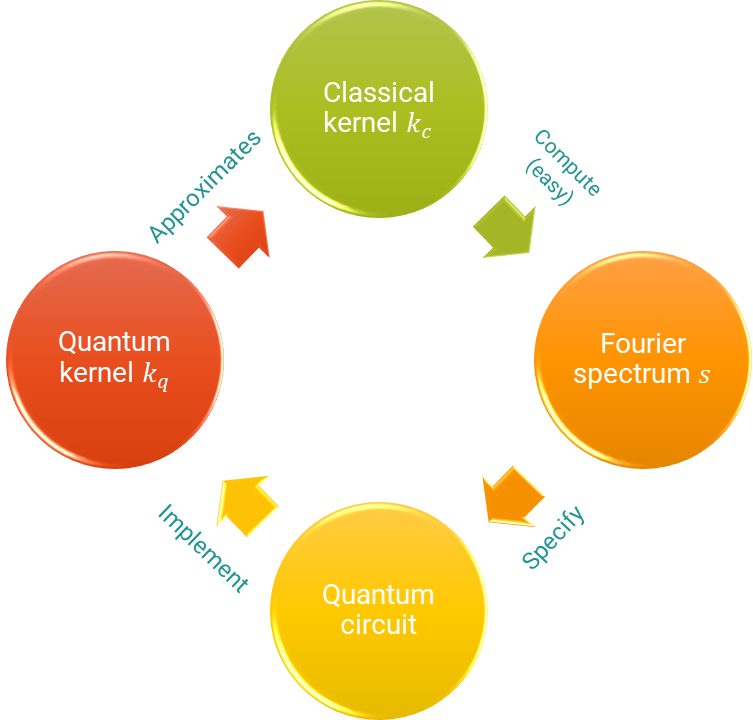
Schematic of the steps covered in this demo.

Kernel-based Machine Learning

We will not be reviewing all the notions of kernels in-depth here. Instead, we only need to know that an entire branch of machine learning revolves around some functions we call kernels. If you’d like to learn more about where these functions come from, why they’re important, and how we can use them (e.g. with PennyLane), check out the following demos, which cover different aspects extensively:

1. Training and evaluating quantum kernels

2. Kernel-based training of quantum models with scikit-learn

For the purposes of this demo, a kernel is a real-valued function of two variables \(k(x_1,x_2)\) from a given data domain \(x_1, x_2\in\mathcal{X}\). In this demo, we’ll deal with real vector spaces as the data domain \(\mathcal{X}\subseteq\mathbb{R}^d\), of some dimension \(d\). A kernel has to be symmetric with respect to exchanging both variables \(k(x_1,x_2) = k(x_2,x_1)\). We also enforce kernels to be positive semi-definite, but let’s avoid getting lost in mathematical lingo. You can trust that all kernels featured in this demo are positive semi-definite.

Shift-invariant kernels

Some kernels fulfill another important restriction, called shift-invariance. Shift-invariant kernels are those whose value doesn’t change if we add a shift to both inputs. Explicitly, for any suitable shift vector \(\zeta\in\mathcal{X}\), shift-invariant kernels are those for which \(k(x_1+\zeta,x_2+\zeta)=k(x_1,x_2)\) holds. Having this property means the function can be written in terms of only one variable, which we call the lag vector \(\delta:=x_1-x_2\in\mathcal{X}\). Abusing notation a bit:

\[k(x_1,x_2)=k(x_1-x_2,0) = k(\delta).\]

For shift-invariant kernels, the exchange symmetry property \(k(x_1,x_2)=k(x_2,x_1)\) translates into reflection symmetry \(k(\delta)=k(-\delta)\). Accordingly, we say \(k\) is an even function.

Warm up: Implementing the Gaussian kernel

First, let’s introduce a simple classical kernel that we will approximate on the quantum computer. Start importing the usual suspects:

import pennylane as qml
from pennylane import numpy as np
import matplotlib.pyplot as plt
import math
np.random.seed(53173)

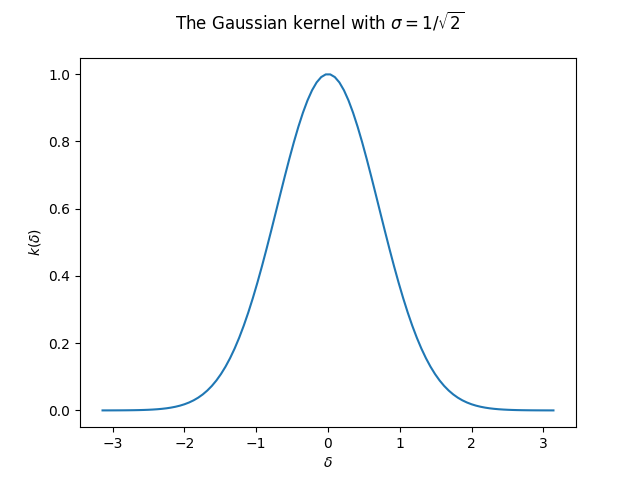
We’ll look at the Gaussian kernel: \(k_\sigma(x_1,x_2):=e^{-\lVert x_1-x_2\rVert^2/2\sigma^2}\). This function is clearly shift-invariant:

\[\begin{split}k_\sigma(x_1+\zeta,x_2+\zeta) &= e^{-\lVert(x_1+\zeta)-(x_2+\zeta)\rVert^2/2\sigma^2} \\ & = e^{-\lVert x_1-x_2\rVert^2/2\sigma^2} \\ & = k_\sigma(x_1,x_2).\end{split}\]

The object of our study will be a simple version of the Gaussian kernel, where we consider \(1\)-dimensional data, so \(\lVert x_1-x_2\rVert^2=(x_1-x_2)^2\). Also, we take \(\sigma=1/\sqrt{2}\) so that we further simplify the exponent. We can always re-introduce it later by rescaling the data. Again, we can write the function in terms of the lag vector only:

\[k(\delta)=e^{-\delta^2}.\]

Now let’s write a few lines to plot the Gaussian kernel:

def gaussian_kernel(delta):
    return math.exp(-delta ** 2)

def make_data(n_samples, lower=-np.pi, higher=np.pi):
    x = np.linspace(lower, higher, n_samples)
    y = np.array([gaussian_kernel(x_) for x_ in x])
    return x,y

X, Y_gaussian = make_data(100)

plt.plot(X, Y_gaussian)
plt.suptitle("The Gaussian kernel with $\sigma=1/\sqrt{2}$")
plt.xlabel("$\delta$")
plt.ylabel("$k(\delta)$")
plt.show();

In this demo, we will consider only this one example. However, the arguments we make and the code we use are also amenable to any kernel with the following mild restrictions:

1. Shift-invariance

2. Normalization \(k(0)=1\).

3. Smoothness (in the sense of a quickly decaying Fourier spectrum).

Note that is a very large class of kernels! And also an important one for practical applications.

Fourier analysis of the Gaussian kernel

The next step will be to find the Fourier spectrum of the Gaussian kernel, which is an easy problem for classical computers. Once we’ve found it, we’ll build a QK that produces a finite Fourier series approximation to that spectrum.

Let’s briefly recall that a Fourier series is the representation of a periodic function using the sine and cosine functions. Fourier analysis tells us that we can write any given periodic function as

\[f(x) = a_0 + \sum_{n=1}^\infty a_n\cos(n\omega_0x) + b_n\sin(n\omega_0x).\]

For that, we only need to find the suitable base frequency \(\omega_0\) and coefficients \(a_0, a_1, \ldots, b_0, b_1,\ldots\).

But the Gaussian kernel is an aperiodic function, whereas the Fourier series only makes sense for periodic functions!

What can we do?!

We can cook up a periodic extension to the Gaussian kernel, for a given period \(2L\) (we take \(L=\pi\) as default):

def Gauss_p(x, L=np.pi):
    # Send x to x_mod in the period around 0
    x_mod = np.mod(x+L, 2*L) - L
    return gaussian_kernel(x_mod)

which we can now plot

x_func = np.linspace(-10, 10, 321)
y_func = [Gauss_p(x) for x in x_func]

plt.plot(x_func, y_func)
plt.xlabel("$\delta$")
plt.suptitle("Periodic extension to the Gaussian kernel")
plt.show();

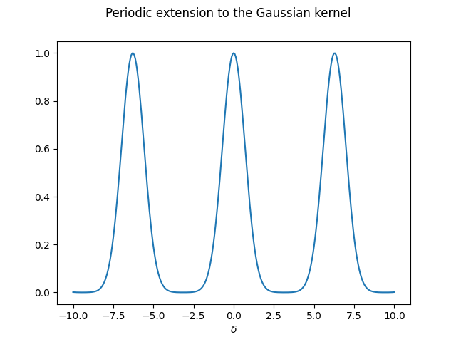
In practice, we would construct several periodic extensions of the aperiodic function, with increasing periods. This way, we can study the behaviour when the period approaches infinity, i.e. the regime where the function stops being periodic.

Next up, how does the Fourier spectrum of such an object look like? We can find out using PennyLane’s fourier module!

from pennylane.fourier import coefficients

The function coefficients computes for us the coefficients of the Fourier series up to a fixed term. One tiny detail here: coefficients returns one complex number \(c_n\) for each frequency \(n\). The real part corresponds to the \(a_n\) coefficient, and the imaginary part to the \(b_n\) coefficient: \(c_n=a_n+ib_n\). Because the Gaussian kernel is an even function, we know that the imaginary part of every coefficient will be zero, so \(c_n=a_n\).

def fourier_p(d):
    """
    We only take the first d coefficients [:d]
    because coefficients() treats the negative frequencies
    as different from the positive ones.
    For real functions, they are the same.
    """
    return np.real(coefficients(Gauss_p, 1, d-1)[:d])

We are restricted to considering only a finite number of Fourier terms. But isn’t that problematic, one may say? Well, maybe. Since we know the Gaussian kernel is a smooth function, we expect that the coefficients converge to \(0\) at some point, and we will only need to consider terms up to this point. Let’s look at the coefficients we obtain by setting a low value for the number of coefficients and then slowly letting it grow:

N = [0]
for n in range(2,7):
    N.append(n)
    F = fourier_p(n)
    plt.plot(N, F, 'x', label='{}'.format(n))

plt.legend()
plt.xlabel("frequency $n$")
plt.ylabel("Fourier coefficient $c_n$")
plt.show();

What do we see? For very small coefficient counts, like \(2\) and \(3\), we see that the last allowed coefficient is still far from \(0\). That’s a very clear indicator that we need to consider more frequencies. At the same time, it seems like starting at \(5\) or \(6\) all the non-zero contributions have already been well captured. This is important for us, since it tells us the minimum number of qubits we should use. One can see that every new qubit doubles the number of frequencies we can use, so for \(n\) qubits, we will have \(2^n\). At minimum of \(6\) frequencies means at least \(3\) qubits, corresponding to \(2^3=8\) frequencies. As we’ll see later, we’ll work with \(5\) qubits, so \(32\) frequencies. That means the spectrum we will be trying to replicate will be the following:

plt.plot(range(32), fourier_p(32), 'x')
plt.xlabel("frequency $n$")
plt.ylabel("Fourier coefficient $c_n$")
plt.suptitle("Fourier spectrum of the Gaussian kernel")
plt.show();

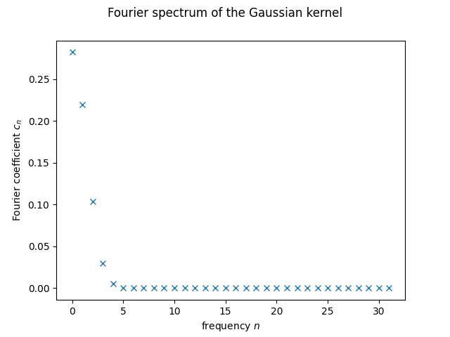
We just need a QK with the same Fourier spectrum!

Designing a suitable QK

Designing a suitable QK amounts to designing a suitable parametrized quantum circuit. Let’s take a moment to refresh the big scheme of things with the following picture:

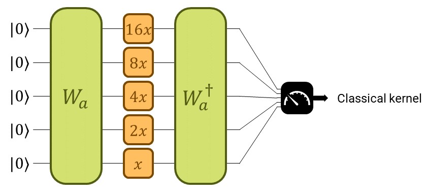
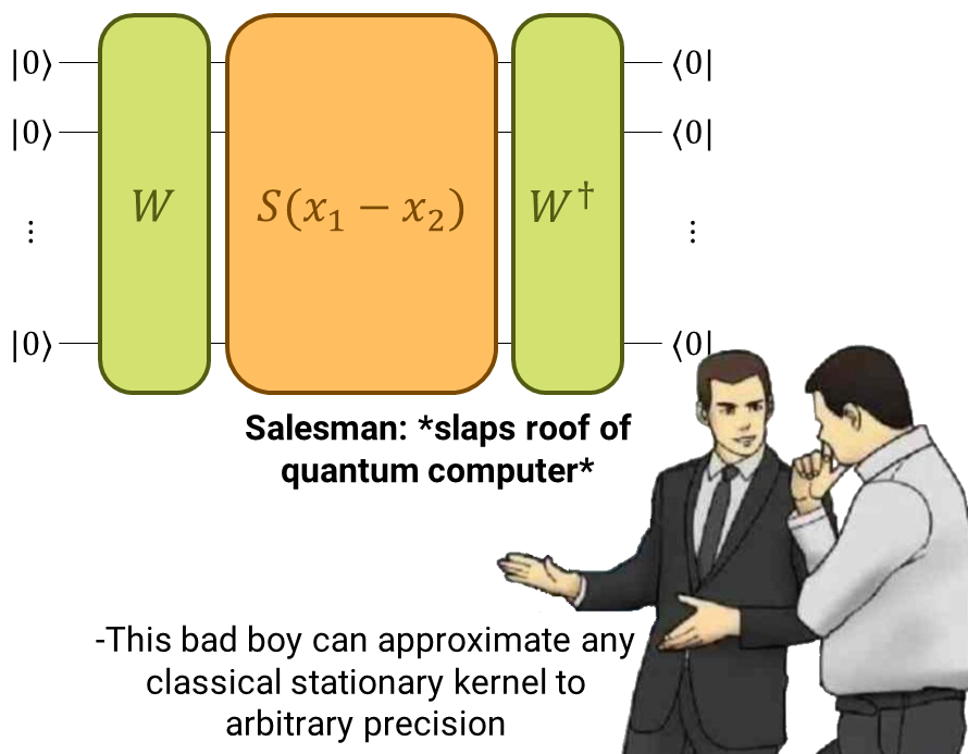
The quantum kernel considered in this demo.

We construct the quantum kernel from a quantum embedding (see the demo on Quantum Embedding Kernels). The quantum embedding circuit will consist of two parts. The first one, trainable, will be a parametrized general state preparation scheme \(W_a\), with parameters \(a\). In the second one, we input the data, denoted by \(S(x)\).

Start with the non-trainable gate we’ll use to encode the data \(S(x)\). It consists of applying one Pauli-\(Z\) rotation to each qubit with rotation parameter \(x\) times some constant \(\vartheta_i\), for the \(i^\text{th}\) qubit.

def S(x, thetas, wires):
    for (i, wire) in enumerate(wires):
        qml.RZ(thetas[i] * x, wires = [wire])

By setting the thetas properly, we achieve the integer-valued spectrum, as required by the Fourier series expansion of a function of period \(2\pi\): \(\{0, 1, \ldots, 2^n-2, 2^n-1\}\), for \(n\) qubits. Some math shows that setting \(\vartheta_i=2^{n-i}\), for \(\{1,\ldots,n\}\) produces the desired outcome.

def make_thetas(n_wires):
    return [2 ** i for i in range(n_wires-1, -1, -1)]

Next, we introduce the only trainable gate we need to make use of. Contrary to the usual Ansätze used in supervised and unsupervised learning, we use a state preparation template called MottonenStatePreparation. This is one option for amplitude encoding already implemented in PennyLane, so we don’t need to code it ourselves. Amplitude encoding is a common way of embedding classical data into a quantum system in QML. The unitary associated to this template transforms the \(\lvert0\rangle\) state into a state with amplitudes \(a=(a_0,a_1,\ldots,a_{2^n-1})\), namely \(\lvert a\rangle=\sum_j a_j\lvert j\rangle\), provided \(\lVert a\rVert^2=1\).

def W(features, wires):
    qml.templates.state_preparations.MottonenStatePreparation(features, wires)

With that, we have the feature map onto the Hilbert space of the quantum computer:

\[\lvert x_a\rangle = S(x)W_a\lvert0\rangle,\]

for a given \(a\), which we will specify later.

Accordingly, we can build the QK corresponding to this feature map as

\[\begin{split}k_a(x_1,x_2) &= \lvert\langle0\rvert W_a^\dagger S^\dagger(x_1) S(x_2)W_a\lvert0\rangle\rvert^2 \\ &= \lvert\langle0\rvert W_a^\dagger S(x_2-x_1) W_a\lvert0\rangle\rvert^2.\end{split}\]

In the code below, the variable amplitudes corresponds to our set \(a\).

def ansatz(x1, x2, thetas, amplitudes, wires):
    W(amplitudes, wires)
    S(x1 - x2, thetas, wires)
    qml.adjoint(W)(amplitudes, wires)

Since this kernel is by construction real-valued, we also have

\[\begin{split}(k_a(x_1,x_2))^\ast &= k_a(x_1,x_2) \\ &= \lvert\langle0\rvert W_a^\dagger S(x_1-x_2) W_a\lvert0\rangle\rvert^2 \\ &= k_a(x_2,x_1).\end{split}\]

Further, this QK is also shift-invariant \(k_a(x_1,x_2) = k_a(x_1+\zeta, x_2+\zeta)\) for any \(\zeta\in\mathbb{R}\). So we can also write it in terms of the lag \(\delta=x_1-x_2\):

\[k_a(\delta) = \lvert\langle0\rvert W_a^\dagger S(\delta)W_a\lvert0\rangle\rvert^2.\]

So far, we only wrote the gate layout for the quantum circuit, no measurement! We need a few more functions for that!

Computing the QK function on a quantum device

Also, at this point, we need to set the number of qubits of our computer. For this example, we’ll use the variable n_wires, and set it to \(5\).

n_wires = 5

We initialize the quantum simulator:

dev = qml.device("default.qubit", wires = n_wires, shots = None)

Next, we construct the quantum node:

@qml.qnode(dev, interface="autograd")
def QK_circuit(x1, x2, thetas, amplitudes):
    ansatz(x1, x2, thetas, amplitudes, wires = range(n_wires))
    return qml.probs(wires = range(n_wires))

Recall that the output of a QK is defined as the probability of obtaining the outcome \(\lvert0\rangle\) when measuring in the computational basis. That corresponds to the \(0^\text{th}\) entry of qml.probs:

def QK_2(x1, x2, thetas, amplitudes):
    return QK_circuit(x1, x2, thetas, amplitudes)[0]

As a couple of quality-of-life improvements, we write a function that implements the QK with the lag \(\delta\) as its argument, and one that implements it on a given set of data:

def QK(delta, thetas, amplitudes):
    return QK_2(delta, 0, thetas, amplitudes)

def QK_on_dataset(deltas, thetas, amplitudes):
    y = np.array([QK(delta, thetas, amplitudes) for delta in deltas])
    return y

This is also a good place to fix the thetas array, so that we don’t forget later.

thetas = make_thetas(n_wires)

Let’s see how this looks like for one particular choice of amplitudes. We need to make sure the array fulfills the normalization conditions.

test_features = np.asarray([1./(1+i) for i in range(2 ** n_wires)])
test_amplitudes = test_features / np.sqrt(np.sum(test_features ** 2))

Y_test = QK_on_dataset(X, thetas, test_amplitudes)

plt.plot(X, Y_test)
plt.xlabel("$\delta$")
plt.suptitle("QK with test amplitudes")
plt.show();

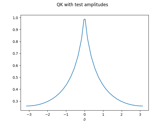
One can see that the stationary kernel with this particular initial state has a decaying spectrum that looks similar to \(1/\lvert x\rvert\) — but not yet like a Gaussian.

How to find the amplitudes emulating a Gaussian kernel

If we knew exactly which amplitudes to choose in order to build a given Fourier spectrum, our job would be done here. However, the equations derived in the literature are not trivial to solve.

As mentioned in the introduction, one could just “learn” this relation, that is, tune the parameters of the quantum kernel in a gradient-based manner until it matches the classical one.

We want to take an intermediate route between analytical solution and black-box optimization. For that, we derive an equation that links the amplitudes to the spectrum we want to construct and then use old-fashioned convex optimization to find the solution. If you are not interested in the details, you can just jump to the last plots of this demo and confirm that we can to emulate the Gaussian kernel using the ansatz for our QK constructed above.

In order to simplify the formulas, we introduce new variables, which we call probabilities \((p_0, p_1, p_2, \ldots, p_{2^n-1})\), and we define as \(p_j=\lvert a_j\rvert^2\). Following the normalization property above, we have \(\sum_j p_j=1\). Don’t get too fond of them, we only need them for this step! Remember we introduced the vector \(a\) for the MottonenStatePreparation as the amplitudes of a quantum state? Then it makes sense that we call its squares probabilities, doesn’t it?

There is a crazy formula that matches the entries of probabilities with the Fourier series of the resulting QK function:

\[\begin{split}\text{probabilities} &\longrightarrow \text{Fourier coefficients} \\ \begin{pmatrix} p_0 \\ p_1 \\ p_2 \\ \vdots \\ p_{2^n-1} \end{pmatrix} &\longmapsto \begin{pmatrix} \sum_{j=0}^{2^n-1} p_j^2 \\ \sum_{j=1}^{2^n-1} p_j p_{j-1} \\ \sum_{j=2}^{2^n-1} p_j p_{j-2} \\ \vdots \\ p_{2^n-1} p_0 \end{pmatrix}\end{split}\]

This looks a bit scary, it follows from expanding the matrix product \(W_a^\dagger S(\delta)W_a\), and then collecting terms according to Fourier basis monomials. In this sense, the formula is general and it applies to any shift-invariant kernel we might want to approximate, not only the Gaussian kernel.

Our goal is to find the set of \(p_j\)’s that produces the Fourier coefficients of a given kernel function (in our case, the Gaussian kernel), namely its spectrum \((s_0, s_1, s_2, \ldots, s_{2^n-1})\). We consider now a slightly different map \(F_s\), for a given spectrum \((s_0, s_1, \ldots, s_{2^n-1})\):

\[\begin{split}F_s: \text{probabilities} &\longrightarrow \text{Difference between Fourier coefficients} \\ \begin{pmatrix} p_0 \\ p_1 \\ p_2 \\ \vdots \\ p_{2^n-1} \end{pmatrix} &\longmapsto \begin{pmatrix} \sum_{j=0}^{2^n-1} p_j^2 - s_0 \\ \sum_{j=1}^{2^n-1} p_j p_{j-1} - s_1 \\ \sum_{j=2}^{2^n-1} p_j p_{j-2} - s_2 \\ \vdots \\ p_{2^n-1}p_0 - s_{2^n-1} \end{pmatrix}.\end{split}\]

If you look at it again, you’ll see that the zero (or solution) of this second map \(F_s\) is precisely the array of probabilities we are looking for. We can write down the first map as:

def predict_spectrum(probabilities):
    d = len(probabilities)
    spectrum = []
    for s in range(d):
        s_ = 0

        for j in range(s, d):
            s_ += probabilities[j] * probabilities[j - s]

        spectrum.append(s_)

    # This is to make the output have the same format as
    # the output of pennylane.fourier.coefficients
    for s in range(1,d):
        spectrum.append(spectrum[d - s])

    return spectrum

And then \(F_s\) is just predict_spectrum minus the spectrum we want to predict:

def F(probabilities, spectrum):
    d = len(probabilities)
    return predict_spectrum(probabilities)[:d] - spectrum[:d]

These closed-form equations allow us to find the solution numerically, using Newton’s method! Newton’s method is a classical one from convex optimization theory. For our case, since the formula is quadratic, we rest assured that we are within the realm of convex functions.

Finding the solution

In order to use Newton’s method we need the Jacobian of \(F_s\).

def J_F(probabilities):
    d = len(probabilities)
    J = np.zeros(shape=(d,d))
    for i in range(d):
        for j in range(d):
            if (i + j < d):
                J[i][j] += probabilities[i + j]
            if(i - j <= 0):
                J[i][j] += probabilities[j - i]
    return J

Showing that this is indeed \(\nabla F_s\) is left as an exercise for the reader. For Newton’s method, we also need an initial guess. Finding a good initial guess requires some tinkering; different problems will benefit from different ones. Here is a tame one that works for the Gaussian kernel.

def make_initial_probabilities(d):
    probabilities = np.ones(d)
    deg = np.array(range(1, d + 1))
    probabilities = probabilities / deg
    return probabilities

probabilities = make_initial_probabilities(2 ** n_wires)

Recall the spectrum we want to match is that of the periodic extension of the Gaussian kernel.

spectrum = fourier_p(2 ** n_wires)

We fix the hyperparameters for Newton’s method:

d = 2 ** n_wires
max_steps = 100
tol = 1.e-20

And we’re good to go!

for step in range(max_steps):
    inc = np.linalg.solve(J_F(probabilities), -F(probabilities, spectrum))
    probabilities = probabilities + inc
    if (step+1) % 10 == 0:
        print("Error norm at step {0:3}: {1}".format(step + 1,
                                               np.linalg.norm(F(probabilities,
                                                                spectrum))))
        if np.linalg.norm(F(probabilities, spectrum)) < tol:
            print("Tolerance trespassed! This is the end.")
            break

Out:

Error norm at step  10: 7.232364210931579e-14
Error norm at step  20: 3.471143367379474e-18
Error norm at step  30: 5.56263347695335e-17
Error norm at step  40: 3.127392492141697e-17
Error norm at step  50: 1.3878213524237504e-17
Error norm at step  60: 3.1237255619435047e-17
Error norm at step  70: 7.742031576522774e-21
Tolerance trespassed! This is the end.

The tolerance we set was fairly low, one should expect good things to come out of this. Let’s have a look at the solution:

plt.plot(range(d), probabilities, 'x')
plt.xlabel("array entry $j$")
plt.ylabel("probabilities $p_j$")
plt.show();

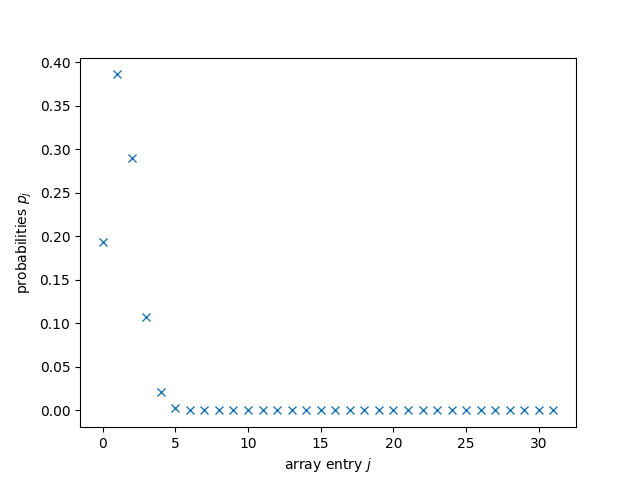
Would you be able to tell whether this is correct? Me neither! But all those probabilities being close to \(0\) should make us fear some of them must’ve turned negative. That would be fatal for us. For MottonenStatePreparation, we’ll need to give amplitudes as one of the arguments, which is the component-wise square root of probabilities. And hence the problem! Even if they are very small values, if any entry of probabilities is negative, the square root will give nan. In order to avoid that, we use a simple thresholding where we replace very small entries by \(0\).

def probabilities_threshold_normalize(probabilities, thresh = 1.e-10):
    d = len(probabilities)
    p_t = probabilities.copy()
    for i in range(d):
        if np.abs(probabilities[i] < thresh):
            p_t[i] = 0.0

    p_t = p_t / np.sum(p_t)

    return p_t

Then, we need to take the square root:

probabilities = probabilities_threshold_normalize(probabilities)
amplitudes = np.sqrt(probabilities)

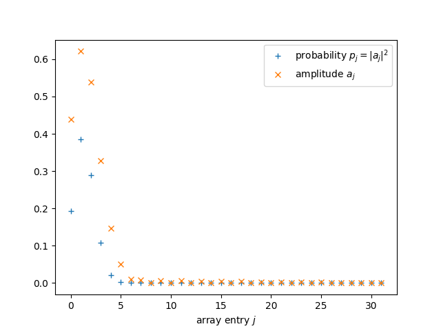
A little plotting never killed nobody

plt.plot(range(d), probabilities, '+', label = "probability $p_j = |a_j|^2$")
plt.plot(range(d), amplitudes, 'x', label = "amplitude $a_j$")
plt.xlabel("array entry $j$")
plt.legend()
plt.show();

Visualizing the solution

And the moment of truth! Does the solution really match the spectrum? We try it first using predict_spectrum only

plt.plot(range(d), fourier_p(d)[:d], '+', label = "Gaussian kernel")
plt.plot(range(d), predict_spectrum(probabilities)[:d], 'x', label = "QK predicted")
plt.xlabel("frequency $n$")
plt.ylabel("Fourier coefficient")
plt.suptitle("Fourier spectrum of the Gaussian kernel")
plt.legend()
plt.show();

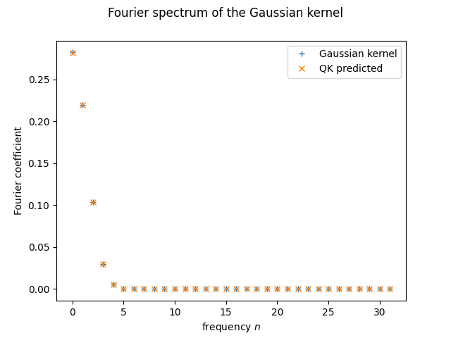
It seems like it does! But as we just said, this is still only the predicted spectrum. We haven’t called the quantum computer at all yet!

Let’s see what happens when we call the function coefficients on the QK function we defined earlier. Good coding practice tells us we should probably turn this step into a function itself, in case it is of use later:

def fourier_q(d, thetas, amplitudes):
    def QK_partial(x):
        squeezed_x = qml.math.squeeze(x)
        return QK(squeezed_x, thetas, amplitudes)
    return np.real(coefficients(QK_partial, 1, d-1))

And with this, we can finally visualize how the Fourier spectrum of the QK function compares to that of the Gaussian kernel:

plt.plot(range(d), fourier_p(d)[:d], '+', label = "Gaussian kernel")
plt.plot(range(d), predict_spectrum(probabilities)[:d], 'x', label="QK predicted")
plt.plot(range(d), fourier_q(d, thetas, amplitudes)[:d], '.', label = "QK computer")
plt.xlabel("frequency $n$")
plt.ylabel("Fourier coefficient")
plt.suptitle("Fourier spectrum of the Gaussian kernel")
plt.legend()
plt.show();

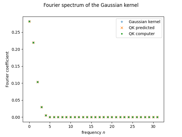
It seems it went well! Matching spectra should mean matching kernel functions, right?

Y_learned = QK_on_dataset(X, thetas, amplitudes)
Y_truth = [Gauss_p(x_) for x_ in X]

plt.plot(X, Y_learned, '-.', label = "QK")
plt.plot(X, Y_truth, '--', label = "Gaussian kernel")
plt.xlabel("$\delta$")
plt.ylabel("$k(\delta)$")
plt.legend()
plt.show();

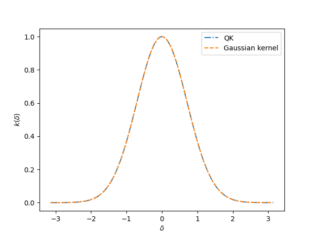
Yeah! We did it!

References

1

Thomas Hubregtsen, David Wierichs, Elies Gil-Fuster, Peter-Jan HS Derks, Paul K Faehrmann, Johannes Jakob Meyer. “Training Quantum Embedding Kernels on Near-Term Quantum Computers”. arXiv preprint arXiv:2105.02276.

2

Maria Schuld, Ryan Sweke, Johannes Jakob Meyer. “The effect of data encoding on the expressive power of variational quantum machine learning models”. Phys. Rev. A 103, 032430, arXiv preprint arXiv:2008.08605.

3

Maria Schuld. “Supervised quantum machine learning models are kernel methods”. arXiv preprint arXiv:2101.11020.

About the author

Elies Gil-Fuster

Elies is a QML researcher in Berlin interested in board games and the maths of data re-uploading PQCs. He was a Xanadu Summer Resident of the first cohort, and you can find more about him at https://eliesgilfuster.eu.

demos/tutorial_classical_kernels

 

Download Python script

 

Download Notebook

 

View on GitHub