Classical shadows

Authors: Roeland Wiersema and Brian Doolittle (Xanadu Residents) — Posted: 14 June 2021. Last updated: 14 June 2021.

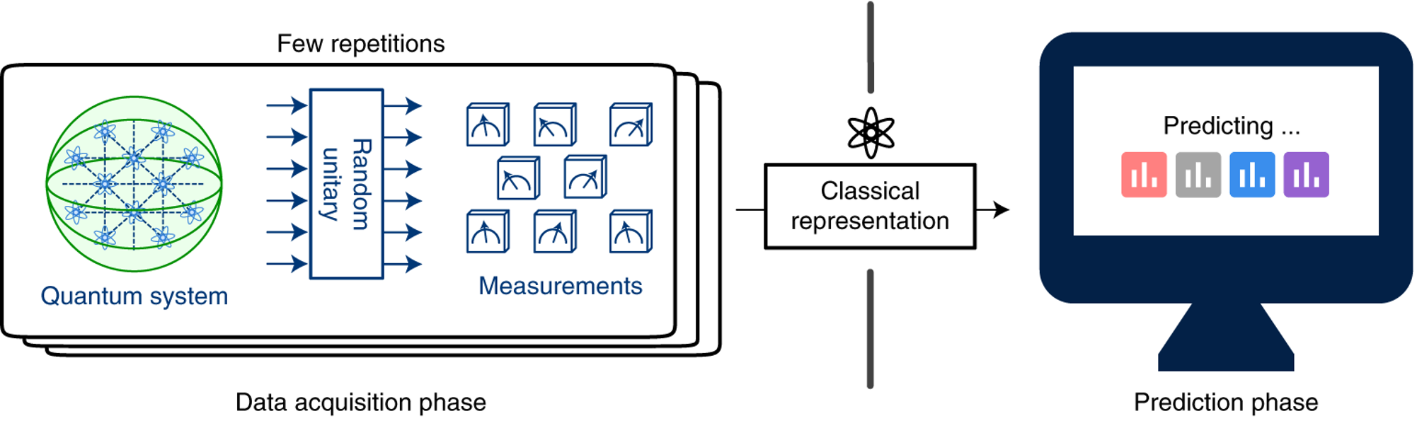
Estimating properties of unknown quantum states is a key objective of quantum information science and technology. For example, one might want to check whether an apparatus prepares a particular target state, or verify that an unknown system is entangled. In principle, any unknown quantum state can be fully characterized by quantum state tomography 1. However, this procedure requires accurate expectation values for a set of observables whose size grows exponentially with the number of qubits. A potential workaround for these scaling concerns is provided by the classical shadow approximation introduced in a recent paper by Huang et al. 2.

The approximation is an efficient protocol for constructing a classical shadow representation of an unknown quantum state. The classical shadow can be used to estimate properties such as quantum state fidelity, expectation values of Hamiltonians, entanglement witnesses, and two-point correlators.

(Image from Huang et al. 2.)

In this demo, we use PennyLane to obtain classical shadows of a quantum state prepared by a quantum circuit, and use them to reconstruct the state and estimate expectation values of observables.

Constructing a Classical Shadow

Classical shadow estimation relies on the fact that for a particular choice of measurement, we can efficiently store snapshots of the state that contain enough information to accurately predict linear functions of observables. Depending on what type of measurements we choose, we have an information-theoretic bound that allows us to control the precision of our estimator.

Let us consider an \(n\)-qubit quantum state \(\rho\) (prepared by a circuit) and apply a random unitary \(U\) to the state:

\[\rho \to U \rho U^\dagger.\]

Next, we measure in the computational basis and obtain a bit string of outcomes \(|b\rangle = |0011\ldots10\rangle\). If the unitaries \(U\) are chosen at random from a particular ensemble, then we can store the reverse operation \(U^\dagger |b\rangle\langle b| U\) efficiently in classical memory. We call this a snapshot of the state. Moreover, we can view the average over these snapshots as a measurement channel:

\[\mathbb{E}\left[U^\dagger |b\rangle\langle b| U\right] = \mathcal{M}(\rho).\]

If the ensemble of unitaries defines a tomographically complete set of measurements, we can invert the channel and reconstruct the state:

\[\rho = \mathbb{E}\left[\mathcal{M}^{-1}\left(U^\dagger |b\rangle\langle b| U \right)\right].\]

If we apply the procedure outlined above \(N\) times, then the collection of inverted snapshots is what we call the classical shadow

\[S(\rho,N) = \left\{\hat{\rho}_1= \mathcal{M}^{-1}\left(U_1^\dagger |b_1\rangle\langle b_1| U_1 \right) ,\ldots, \hat{\rho}_N= \mathcal{M}^{-1}\left(U_N^\dagger |b_N\rangle\langle b_N| U_N \right) \right\}.\]

The inverted channel is not physical, i.e., it is not completely postive and trace preserving (CPTP). However, this is of no concern to us, since all we care about is efficiently applying this inverse channel to the observed snapshots as a post-processing step.

Since the shadow approximates \(\rho\), we can now estimate any observable with the empirical mean:

\[\langle O \rangle = \frac{1}{N}\sum_i \text{Tr}{\hat{\rho}_i O}.\]

Note that the classical shadow is independent of the observables we want to estimate, as \(S(\rho,N)\) contains only information about the state!

Furthermore, the authors of 2 prove that with a shadow of size \(N\), we can predict \(M\) arbitary linear functions \(\text{Tr}{O_1\rho},\ldots,\text{Tr}{O_M \rho}\) up to an additive error \(\epsilon\) if \(N\geq \mathcal{O}\left(\log{M} \max_i ||O_i||^2_{\text{shadow}}/\epsilon^2\right)\). The shadow norm \(||O_i||^2_{\text{shadow}}\) depends on the unitary ensemble that is chosen.

Two different ensembles can be considered for selecting the random unitaries \(U\):

1. Random \(n\)-qubit Clifford circuits.

2. Tensor products of random single-qubit Clifford circuits.

Although ensemble 1 leads to the most powerful estimators, it comes with serious practical limitations since \(n^2 / \log(n)\) entangling gates are required to sample the Clifford circuit. The snapshots of both ensembles can be stored efficiently using the stabilizer formalism 3. Single-qubit Clifford circuits rotate the measurement basis to one of the Pauli eigenbases, so ensemble 2 is equivalent to measuring single shots of single-qubit Pauli observables on all qubits. For the purposes of this demo we focus on ensemble 2, which is a more NISQ-friendly approach.

This ensemble comes with a significant drawback: the shadow norm \(||O_i||^2_{\text{shadow}}\) becomes dependent on the locality \(k\) of the observables that we want to estimate:

\[||O_i||^2_{\text{shadow}} \leq 4^k ||O_i||_\infty^2.\]

Say that we want to estimate the single expectation value of a Pauli observable \(\langle X_1 \otimes X_2 \otimes \ldots \otimes X_n \rangle\). Estimating this from repeated measurements would require \(1/\epsilon^2\) samples, whereas we would need an exponentially large shadow due to the \(4^n\) appearing in the bound. Therefore, classical shadows based on Pauli measurements only offer an advantage when we have to measure a large number of observables with modest locality.

We will now demonstrate how to obtain classical shadows using PennyLane.

import pennylane as qml
import pennylane.numpy as np
import matplotlib.pyplot as plt
import time

np.random.seed(666)

A classical shadow is a collection of \(N\) individual snapshots \(\hat{\rho}_i\). Each snapshot is obtained with the following procedure:

1. The quantum state \(\rho\) is prepared with a circuit.

2. A unitary \(U\) is randomly selected from the ensemble and applied to \(\rho\).

3. A computational basis measurement is performed.

4. The snapshot is recorded as the observed eigenvalue \(1,-1\) for \(|0\rangle,|1\rangle\), respectively, and the index of the randomly selected unitary \(U\).

To obtain a classical shadow using PennyLane, we design the calculate_classical_shadow function below. This function obtains a classical shadow for the state prepared by an input circuit_template.

def calculate_classical_shadow(circuit_template, params, shadow_size, num_qubits):
    """
    Given a circuit, creates a collection of snapshots consisting of a bit string
    and the index of a unitary operation.

    Args:
        circuit_template (function): A Pennylane QNode.
        params (array): Circuit parameters.
        shadow_size (int): The number of snapshots in the shadow.
        num_qubits (int): The number of qubits in the circuit.

    Returns:
        Tuple of two numpy arrays. The first array contains measurement outcomes (-1, 1)
        while the second array contains the index for the sampled Pauli's (0,1,2=X,Y,Z).
        Each row of the arrays corresponds to a distinct snapshot or sample while each
        column corresponds to a different qubit.
    """
    # applying the single-qubit Clifford circuit is equivalent to measuring a Pauli
    unitary_ensemble = [qml.PauliX, qml.PauliY, qml.PauliZ]

    # sample random Pauli measurements uniformly, where 0,1,2 = X,Y,Z
    unitary_ids = np.random.randint(0, 3, size=(shadow_size, num_qubits))
    outcomes = np.zeros((shadow_size, num_qubits))

    for ns in range(shadow_size):
        # for each snapshot, add a random Pauli observable at each location
        obs = [unitary_ensemble[int(unitary_ids[ns, i])](i) for i in range(num_qubits)]
        outcomes[ns, :] = circuit_template(params, observable=obs)

    # combine the computational basis outcomes and the sampled unitaries
    return (outcomes, unitary_ids)

As an example, we demonstrate how to use calculate_classical_shadow and check its performance as the number of snapshots increases. First, we will create a two-qubit device and a circuit that applies an RY rotation to each qubit.

num_qubits = 2

# set up a two-qubit device with shots = 1 to ensure that we only get a single measurement
dev = qml.device("default.qubit", wires=num_qubits, shots=1)


# simple circuit to prepare rho
@qml.qnode(dev)
def local_qubit_rotation_circuit(params, **kwargs):
    observables = kwargs.pop("observable")
    for w in dev.wires:
        qml.RY(params[w], wires=w)

    return [qml.expval(o) for o in observables]


# arrays in which to collect data
elapsed_times = []
shadows = []

# collecting shadows and elapsed times
params = np.random.randn(2)
for num_snapshots in [10, 100, 1000, 10000]:
    start = time.time()
    shadow = calculate_classical_shadow(
        local_qubit_rotation_circuit, params, num_snapshots, num_qubits
    )
    elapsed_times.append(time.time() - start)
    shadows.append(shadow)

# printing out the smallest shadow as an example
print(shadows[0][0])
print(shadows[0][1])

Out:

[[ 1.  1.]
 [ 1.  1.]
 [ 1.  1.]
 [ 1.  1.]
 [ 1.  1.]
 [ 1.  1.]
 [ 1. -1.]
 [ 1.  1.]
 [ 1.  1.]
 [-1. -1.]]
[[2 2]
 [1 2]
 [0 1]
 [2 0]
 [0 2]
 [1 0]
 [2 0]
 [1 2]
 [0 1]
 [1 1]]

Observe that the shadow simply consists of two matrices. Each qubit corresponds to a different column. The first matrix describes outcome of the measurement while the second matrix indexes the measurement applied to each qubit. We now plot the computation times taken to acquire the shadows.

plt.plot([10, 100, 1000, 10000], elapsed_times)
plt.title("Time taken to obtain a classical shadow from a two-qubit state")
plt.xlabel("Number of Snapshots in Shadow")
plt.ylabel("Elapsed Time")
plt.show()

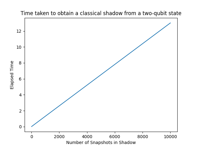
As one might expect, the computation time increases linearly with the number of snapshots. This linear scaling is useful for predicting the length of time required to obtain a sufficient number of snapshots for observable estimation.

State Reconstruction from a Classical Shadow

To verify that the classical shadow approximates the exact state that we want to estimate, we tomographically reconstruct the original quantum state \(\rho\) from a classical shadow. Remember that we can approximate \(\rho\) by averaging over the snapshots and applying the inverse measurement channel,

\[\rho = \mathbb{E}\left[\mathcal{M}^{-1}(U^{\dagger}|\hat{b}\rangle\langle\hat{b}|U)\right].\]

The expectation \(\mathbb{E}[\cdot]\) describes the average over the measurement outcomes \(|b\rangle\) and the sampled unitaries. Inverting the measurement channel may seem formidable at first, however, Huang et al. 2 show that for Pauli measurements we end up with a rather convenient expression,

\[\rho=\mathbb{E}[\hat{\rho}], \quad \text{where} \quad \hat{\rho} = \bigotimes_{j=1}^n(3U^{\dagger}_j|\hat{b}_j\rangle\langle\hat{b}_j|U_j-\mathbb{I}).\]

Here \(\hat{\rho}\) is a snapshot state reconstructed from a single sample in the classical shadow, and \(\rho\) is the average over all snapshot states \(\hat{\rho}\) in the shadow.

To implement the state reconstruction of \(\rho\) in PennyLane, we develop the shadow_state_reconstruction function.

def snapshot_state(b_list, obs_list):
    """
    Helper function for `shadow_state_reconstruction` that reconstructs
     a state from a single snapshot in a shadow.

    Implements Eq. (S44) from https://arxiv.org/pdf/2002.08953.pdf

    Args:
        b_list (array): The list of classical outcomes for the snapshot.
        obs_list (array): Indices for the applied Pauli measurement.

    Returns:
        Numpy array with the reconstructed snapshot.
    """
    num_qubits = len(b_list)

    # computational basis states
    zero_state = np.array([[1, 0], [0, 0]])
    one_state = np.array([[0, 0], [0, 1]])

    # local qubit unitaries
    phase_z = np.array([[1, 0], [0, -1j]], dtype=complex)
    hadamard = qml.matrix(qml.Hadamard(0))
    identity = qml.matrix(qml.Identity(0))

    # undo the rotations that were added implicitly to the circuit for the Pauli measurements
    unitaries = [hadamard, hadamard @ phase_z, identity]

    # reconstructing the snapshot state from local Pauli measurements
    rho_snapshot = [1]
    for i in range(num_qubits):
        state = zero_state if b_list[i] == 1 else one_state
        U = unitaries[int(obs_list[i])]

        # applying Eq. (S44)
        local_rho = 3 * (U.conj().T @ state @ U) - identity
        rho_snapshot = np.kron(rho_snapshot, local_rho)

    return rho_snapshot


def shadow_state_reconstruction(shadow):
    """
    Reconstruct a state approximation as an average over all snapshots in the shadow.

    Args:
        shadow (tuple): A shadow tuple obtained from `calculate_classical_shadow`.

    Returns:
        Numpy array with the reconstructed quantum state.
    """
    num_snapshots, num_qubits = shadow[0].shape

    # classical values
    b_lists, obs_lists = shadow

    # Averaging over snapshot states.
    shadow_rho = np.zeros((2 ** num_qubits, 2 ** num_qubits), dtype=complex)
    for i in range(num_snapshots):
        shadow_rho += snapshot_state(b_lists[i], obs_lists[i])

    return shadow_rho / num_snapshots

Example: Reconstructing a Bell State

First, we construct a single-shot, 'default.qubit' device and define the bell_state_circuit QNode to construct and measure a Bell state.

num_qubits = 2

dev = qml.device("default.qubit", wires=num_qubits, shots=1)


# circuit to create a Bell state and measure it in
# the bases specified by the 'observable' keyword argument.
@qml.qnode(dev)
def bell_state_circuit(params, **kwargs):
    observables = kwargs.pop("observable")

    qml.Hadamard(0)
    qml.CNOT(wires=[0, 1])

    return [qml.expval(o) for o in observables]

Then, construct a classical shadow consisting of 1000 snapshots.

num_snapshots = 1000
params = []

shadow = calculate_classical_shadow(
    bell_state_circuit, params, num_snapshots, num_qubits
)
print(shadow[0])
print(shadow[1])

Out:

[[ 1. -1.]
 [ 1. -1.]
 [ 1. -1.]
 ...
 [ 1. -1.]
 [-1.  1.]
 [ 1.  1.]]
[[1 0]
 [0 1]
 [2 0]
 ...
 [1 1]
 [1 1]
 [0 2]]

To reconstruct the Bell state we use shadow_state_reconstruction.

shadow_state = shadow_state_reconstruction(shadow)
print(np.round(shadow_state, decimals=6))

Out:

[[ 0.50275+0.j       0.0285 -0.02325j  0.06375+0.j       0.4995 -0.00675j]
 [ 0.0285 +0.02325j -0.01925+0.j       0.027  -0.00675j -0.04425-0.018j  ]
 [ 0.06375-0.j       0.027  +0.00675j -0.05675+0.j       0.006  +0.00375j]
 [ 0.4995 +0.00675j -0.04425+0.018j    0.006  -0.00375j  0.57325+0.j     ]]

Note the resemblance to the exact Bell state density matrix.

bell_state = np.array([[0.5, 0, 0, 0.5], [0, 0, 0, 0], [0, 0, 0, 0], [0.5, 0, 0, 0.5]])

To measure the closeness we can use the operator norm.

def operator_2_norm(R):
    """
    Calculate the operator 2-norm.

    Args:
        R (array): The operator whose norm we want to calculate.

    Returns:
        Scalar corresponding to the norm.
    """
    return np.sqrt(np.trace(R.conjugate().transpose() @ R))


# Calculating the distance between ideal and shadow states.
operator_2_norm(bell_state - shadow_state)

Out:

(0.16156422871415568+0j)

Finally, we see how the approximation improves as we increase the number of snapshots. We run the estimator 10 times for each \(N\).

number_of_runs = 10
snapshots_range = [100, 1000, 6000]
distances = np.zeros((number_of_runs, len(snapshots_range)))

# run the estimation multiple times so that we can include error bars
for i in range(number_of_runs):
    for j, num_snapshots in enumerate(snapshots_range):
        shadow = calculate_classical_shadow(
            bell_state_circuit, params, num_snapshots, num_qubits
        )
        shadow_state = shadow_state_reconstruction(shadow)

        distances[i, j] = np.real(operator_2_norm(bell_state - shadow_state))

plt.errorbar(
    snapshots_range,
    np.mean(distances, axis=0),
    yerr=np.std(distances, axis=0),
)
plt.title("Distance between Ideal and Shadow Bell States")
plt.xlabel("Number of Snapshots")
plt.ylabel("Distance")
plt.show()

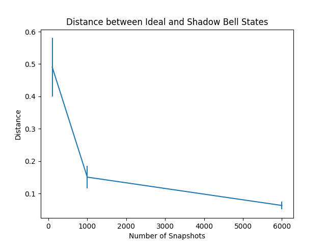
As expected, when the number of snapshots increases, the state reconstruction becomes closer to the ideal state.

Estimating Pauli Observables with Classical Shadows

We have confirmed that classical shadows can be used to reconstruct the state. However, the goal of classical shadows is not to perform full tomography, which takes an exponential amount of resources. Instead, we want to use the shadows to efficiently calculate linear functions of a quantum state. To do this, we write a function estimate_shadow_observable that takes in the previously constructed shadow \(S(\rho, N)=[\hat{\rho}_1,\hat{\rho}_2,\ldots,\hat{\rho}_N]\), and estimates any observable via a median of means estimation. This makes the estimator more robust to outliers and is required to formally prove the aforementioned theoretical bound. The procedure is simple: split up the shadow into \(K\) equally sized chunks and estimate the mean for each of these chunks,

\[\langle O_{(k)}\rangle = \text{Tr}\{O \hat{\rho}_{(k)}\} \quad \text{and} \quad \hat{\rho}_{(k)} = \frac{1}{ \lfloor N/K \rfloor } \sum_{i=(k-1)\lfloor N/K \rfloor + 1}^{k \lfloor N/K \rfloor } \hat{\rho}_i.\]

The median of means estimator is then simply the median of this set

\[\langle O\rangle = \text{median}\{\langle O_{(1)} \rangle,\ldots, \langle O_{(K)} \rangle \}.\]

Note that the shadow bound has a failure probability \(\delta\). By choosing the number of splits \(K\) to be suitably large, we can exponentially suppress this failure probability. Assume now that \(O=\bigotimes_j^n P_j\), where \(P_j \in \{I, X, Y, Z\}\). To efficiently calculate the estimator for \(O\), we look at a single snapshot outcome and plug in the inverse measurement channel:

\[\begin{split}\text{Tr}\{O\hat{\rho}_i\} &= \text{Tr}\{\bigotimes_{j=1}^n P_j (3U^{\dagger}_j|\hat{b}_j\rangle\langle\hat{b}_j|U_j-\mathbb{I})\}\\ &= \prod_j^n \text{Tr}\{ 3 P_j U^{\dagger}_j|\hat{b}_j\rangle\langle\hat{b}_j|U_j\}.\end{split}\]

Due to the orthogonality of the Pauli operators, this evaluates to \(\pm 3\) if \(P_j\) is the corresponding measurement basis \(U_j\) and 0 otherwise. Hence if a single \(U_j\) in the snapshot does not match the one in \(O\), the whole product evaluates to zero. As a result, calculating the mean estimator can be reduced to counting the number of exact matches in the shadow with the observable, and multiplying with the appropriate sign. Below, we develop the function estimate_shadow_obervable to estimate any observable given a classical shadow.

def estimate_shadow_obervable(shadow, observable, k=10):
    """
    Adapted from https://github.com/momohuang/predicting-quantum-properties
    Calculate the estimator E[O] = median(Tr{rho_{(k)} O}) where rho_(k)) is set of k
    snapshots in the shadow. Use median of means to ameliorate the effects of outliers.

    Args:
        shadow (tuple): A shadow tuple obtained from `calculate_classical_shadow`.
        observable (qml.Observable): Single PennyLane observable consisting of single Pauli
            operators e.g. qml.PauliX(0) @ qml.PauliY(1).
        k (int): number of splits in the median of means estimator.

    Returns:
        Scalar corresponding to the estimate of the observable.
    """
    shadow_size, num_qubits = shadow[0].shape

    # convert Pennylane observables to indices
    map_name_to_int = {"PauliX": 0, "PauliY": 1, "PauliZ": 2}
    if isinstance(observable, (qml.PauliX, qml.PauliY, qml.PauliZ)):
        target_obs, target_locs = np.array(
            [map_name_to_int[observable.name]]
        ), np.array([observable.wires[0]])
    else:
        target_obs, target_locs = np.array(
            [map_name_to_int[o.name] for o in observable.obs]
        ), np.array([o.wires[0] for o in observable.obs])

    # classical values
    b_lists, obs_lists = shadow
    means = []

    # loop over the splits of the shadow:
    for i in range(0, shadow_size, shadow_size // k):

        # assign the splits temporarily
        b_lists_k, obs_lists_k = (
            b_lists[i: i + shadow_size // k],
            obs_lists[i: i + shadow_size // k],
        )

        # find the exact matches for the observable of interest at the specified locations
        indices = np.all(obs_lists_k[:, target_locs] == target_obs, axis=1)

        # catch the edge case where there is no match in the chunk
        if sum(indices) > 0:
            # take the product and sum
            product = np.prod(b_lists_k[indices][:, target_locs], axis=1)
            means.append(np.sum(product) / sum(indices))
        else:
            means.append(0)

    return np.median(means)

Next, we can define a function that calculates the number of samples required to get an error \(\epsilon\) on our estimator for a given set of observables.

def shadow_bound(error, observables, failure_rate=0.01):
    """
    Calculate the shadow bound for the Pauli measurement scheme.

    Implements Eq. (S13) from https://arxiv.org/pdf/2002.08953.pdf

    Args:
        error (float): The error on the estimator.
        observables (list) : List of matrices corresponding to the observables we intend to
            measure.
        failure_rate (float): Rate of failure for the bound to hold.

    Returns:
        An integer that gives the number of samples required to satisfy the shadow bound and
        the chunk size required attaining the specified failure rate.
    """
    M = len(observables)
    K = 2 * np.log(2 * M / failure_rate)
    shadow_norm = (
        lambda op: np.linalg.norm(
            op - np.trace(op) / 2 ** int(np.log2(op.shape[0])), ord=np.inf
        )
        ** 2
    )
    N = 34 * max(shadow_norm(o) for o in observables) / error ** 2
    return int(np.ceil(N * K)), int(K)

Example: Estimating a simple set of observables

Here, we give an example for estimating multiple observables on a 10-qubit circuit. We first create a simple circuit

num_qubits = 10
dev = qml.device("default.qubit", wires=num_qubits, shots=1)


def circuit_base(params, **kwargs):
    observables = kwargs.pop("observable")
    for w in range(num_qubits):
        qml.Hadamard(wires=w)
        qml.RY(params[w], wires=w)
    for w in dev.wires[:-1]:
        qml.CNOT(wires=[w, w + 1])
    for w in dev.wires:
        qml.RZ(params[w + num_qubits], wires=w)
    return [qml.expval(o) for o in observables]


circuit = qml.QNode(circuit_base, dev)

params = np.random.randn(2 * num_qubits)

Next, we define our set of observables

\[O = \sum_{i=0}^{n-1} X_i X_{i+1} + Y_i Y_{i+1} + Z_i Z_{i+1}.\]

list_of_observables = (
        [qml.PauliX(i) @ qml.PauliX(i + 1) for i in range(num_qubits - 1)]
        + [qml.PauliY(i) @ qml.PauliY(i + 1) for i in range(num_qubits - 1)]
        + [qml.PauliZ(i) @ qml.PauliZ(i + 1) for i in range(num_qubits - 1)]
)

With the shadow_bound function, we calculate how many shadows we need to ensure that the absolute error of all individual terms in \(O\) satisfies

\[|\langle{O_i}\rangle_{shadow} - \langle{O_i}\rangle_{exact}| \leq \epsilon\]

for all \(1\leq i \leq M\).

shadow_size_bound, k = shadow_bound(
    error=2e-1, observables=[qml.matrix(o) for o in list_of_observables]
)
shadow_size_bound

Out:

14611

We verify the bound by considering a grid of errors \(\epsilon_i\) and checking that \(|\langle{O_i}\rangle_{shadow} - \langle{O_i}\rangle_{exact}|\) stays below this value for the shadow size calculated in shadow_bound. First, we get the classical shadow estimate.

# create a grid of errors
epsilon_grid = [1 - 0.1 * x for x in range(9)]
shadow_sizes = []
estimates = []

for error in epsilon_grid:
    # get the number of samples needed so that the absolute error < epsilon.
    shadow_size_bound, k = shadow_bound(
        error=error, observables=[qml.matrix(o) for o in list_of_observables]
    )
    shadow_sizes.append(shadow_size_bound)
    print(f"{shadow_size_bound} samples required ")
    # calculate a shadow of the appropriate size
    shadow = calculate_classical_shadow(circuit, params, shadow_size_bound, num_qubits)

    # estimate all the observables in O
    estimates.append([estimate_shadow_obervable(shadow, o, k=k) for o in list_of_observables])

Out:

585 samples required
722 samples required
914 samples required
1193 samples required
1624 samples required
2338 samples required
3653 samples required
6494 samples required
14611 samples required

Then, we calculate the ground truth by changing the device backend.

dev_exact = qml.device("default.qubit", wires=num_qubits)
# change the simulator to be the exact one.
circuit = qml.QNode(circuit_base, dev_exact)

expval_exact = [
    circuit(params, observable=[o]) for o in list_of_observables
]

Finally, we plot the errors \(|\langle{O_i}\rangle_{shadow} - \langle{O_i}\rangle_{exact}|\) for all individual terms in \(O\). We expect that these errors are always smaller than \(\epsilon\).

for j, error in enumerate(epsilon_grid):
    plt.scatter(
        [shadow_sizes[j] for _ in estimates[j]],
        [np.abs(obs - estimates[j][i]) for i, obs in enumerate(expval_exact)],
        marker=".",
    )
plt.plot(
    shadow_sizes,
    [e for e in epsilon_grid],
    linestyle="--",
    color="gray",
    label=rf"$\epsilon$",
    marker=".",
)
plt.xlabel(r"$N$ (Shadow size) ")
plt.ylabel(r"$|\langle O_i \rangle_{exact} - \langle O_i \rangle_{shadow}|$")
plt.legend()
plt.show()

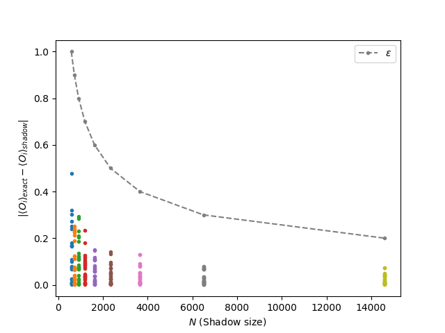
The points in the plot indicate the individual errors for all \(O_i\) at a given shadow size. The dashed line represents the error threshold that these points must stay under to satisfy the bound. As expected, the bound is satisfied for all \(O_i\) and the errors decrease with the size of the shadow.

To conclude, we have shown that classical shadows can be used to reconstruct quantum states and estimate expectation values of observables. This is but the tip of the iceberg of what is possible with this technique. In the original work 2, the authors estimate fidelities, calculate entanglement witnesses, and even find a way to approximate the von Neumann entropy. These applications illustrate the potential power of classical shadows for the characterization of quantum systems.

References

1

G. Mauro D’Ariano, Matteo G.A. Paris, Massimiliano F. Sacchi, “Quantum Tomography”, Advances in Imaging and Electron Physics, 128 (2003): 205-308.

2(1,2,3,4,5)

Huang, Hsin-Yuan, Richard Kueng, and John Preskill, “Predicting many properties of a quantum system from very few measurements”, Nature Physics 16.10 (2020): 1050-1057.

3

Gottesman, Daniel, “Stabilizer Codes and Quantum Error Correction”, Ph.D. thesis, Caltech, eprint quantph/9705052.

About the authors

Roeland Wiersema

Roeland is a PhD student at the university of Waterloo and the Vector Institute doing research in the field of variational quantum computing for quantum many-body simulation.

Brian Doolittle

Brian is a Physics PhD Candidate at the University of Illinois at Urbana-Champaign. Their research focuses upon using variational optimization to better understand quantum communication networks.

demos/tutorial_classical_shadows

 

Download Python script

 

Download Notebook

 

View on GitHub