Note
Click here to download the full example code
Quantum computation with neutral atoms
Author: Nathan Killoran — Posted: 13 October 2020. Last updated: 21 January 2021.
Quantum computing architectures come in many flavours: superconducting qubits, ion traps, photonics, silicon, and more. One very interesting physical substrate is neutral atoms. These quantum devices have some basic similarities to ion traps. Ion-trap devices make use of atoms that have an imbalance between protons (positively charged) and electrons (negatively charged). Neutral atoms, on the other hand, have an equal number of protons and electrons.
In neutral-atom systems, the individual atoms can be easily programmed into various two- or three-dimensional configurations. Like ion-trap systems, individual qubits can be encoded into the energy levels of the atoms. The qubits thus retain the three-dimensional geometry of their host atoms. Qubits that are nearby in space can be programmed to interact with one another via two-qubit gates. This opens up some tantalizing possibilities for exotic quantum-computing circuit topologies.
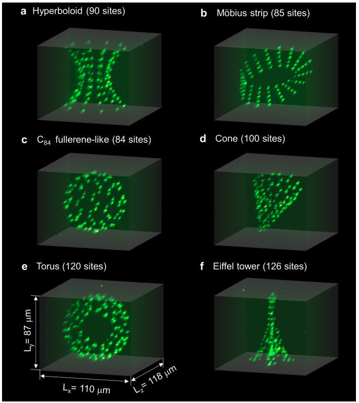
Neutral atoms (green dots) arranged in various configurations. These atoms can be used to encode qubits and carry out quantum computations. Image originally from 1.
The startup Pasqal is one of the companies working to bring neutral-atom quantum computing devices to the world. To support this new class of devices, Pasqal has contributed some new features to the quantum software library Cirq.
In this demo, we will use PennyLane, Cirq, and TensorFlow to show off the unique abilities of neutral atom devices, leveraging them to make a variational quantum circuit which has a very unique topology: the Eiffel tower. Specifically, we will build a simple toy circuit whose qubits are arranged like the Eiffel tower. The girders between the points on the tower will represent two-qubit gates, with the final output of our variational circuit coming at the very peak of the tower.
Let’s get to it!
Note
To run this demo locally, you will need to install Cirq, (version >= 0.9.1), and the PennyLane-cirq plugin (version >= 0.13). You will also need to download a copy of the data, which is available here.
Building the Eiffel tower
Our first step will be to load and visualize the data for the Eiffel tower configuration, which was generously provided by the team at Pasqal. (If running locally, the line below should be updated with the local path where you have saved the downloaded data).
import numpy as np
coords = np.loadtxt("pasqal/Eiffel_tower_data.dat")
xs = coords[:,0]
ys = coords[:,1]
zs = coords[:,2]

import matplotlib.pyplot as plt
fig = plt.figure()
ax = fig.add_subplot(111, projection='3d')
ax.view_init(40, 15)
fig.subplots_adjust(left=0, right=1, bottom=0, top=1)
ax.set_xlim(-20, 20)
ax.set_ylim(-20, 20)
ax.set_zlim(-40, 10)
plt.axis('off')
ax.scatter(xs, ys, zs, c='g',alpha=0.3)
plt.show();
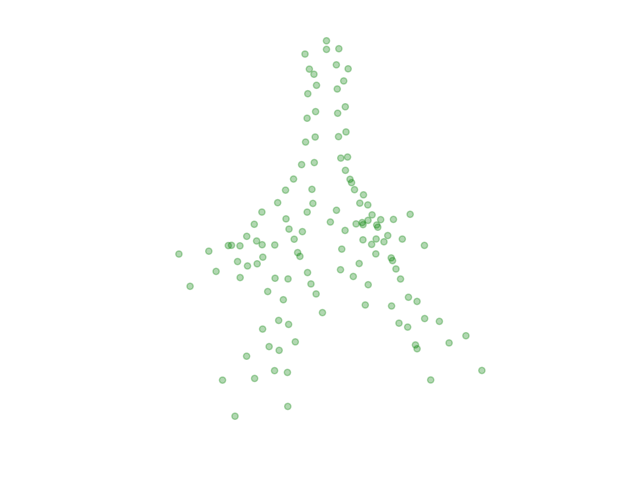
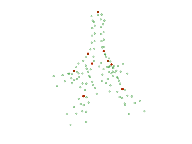
This dataset contains 126 points. Each point represents a distinct neutral-atom qubit. Simulating this many qubits would be outside the reach of Cirq’s built-in simulators, so for this demo, we will pare down to just 9 points, evenly spaced around the tower. These are highlighted in red below.
fig = plt.figure()
ax = fig.add_subplot(111, projection='3d')
ax.view_init(40, 15)
fig.subplots_adjust(left=0, right=1, bottom=0, top=1)
ax.set_xlim(-20, 20)
ax.set_ylim(-20, 20)
ax.set_zlim(-40, 10)
plt.axis('off')
ax.scatter(xs, ys, zs, c='g', alpha=0.3)

base_mask = [3, 7, 11, 15]
qubit_mask = [48, 51, 60, 63, 96, 97, 98, 99, 125]
input_coords = coords[base_mask]  # we'll need this for a plot later
qubit_coords = coords[qubit_mask]

subset_xs = qubit_coords[:, 0]
subset_ys = qubit_coords[:, 1]
subset_zs = qubit_coords[:, 2]
ax.scatter(subset_xs, subset_ys, subset_zs, c='r', alpha=1.0)
plt.show();
Converting to Cirq qubits
Our next step will be to convert these datapoints into objects that
Cirq understands as qubits. For neutral-atom devices in Cirq, we can use the
ThreeDQubit class, which carries information about the three-dimensional
arrangement of the qubits.
Now, neutral-atom devices come with some physical restrictions. Specifically, in a particular three-dimensional configuration, qubits that are too distant from one another can’t easily interact. Instead, there is a notion of a control radius; any atoms which are within the system’s control radius can interact with one another. Qubits separated by a distance larger than the control radius cannot interact.
In order to allow our Eiffel tower qubits to interact with one another more easily, we will artificially scale some dimensions when placing the atoms.
from cirq_pasqal import ThreeDQubit
xy_scale = 1.5
z_scale = 0.75
qubits = [ThreeDQubit(xy_scale * x, xy_scale * y, z_scale * z)
                for x, y, z in qubit_coords]
To simulate a neutral-atom quantum computation, we can use the
"cirq.pasqal" device, available via the
PennyLane-Cirq plugin.
We will need to provide this device with the ThreeDQubit object that we created
above. We also need to instantiate the device with a fixed control radius.
import pennylane as qml

num_wires = len(qubits)
control_radius = 32.4
dev = qml.device("cirq.pasqal", control_radius=control_radius,
                 qubits=qubits, wires=num_wires)
Creating a quantum circuit
We will now make a variational circuit out of the Eiffel tower configuration from above. Each of the 9 qubits we are using can be thought of as a single wire in a quantum circuit. We will cause these qubits to interact by applying a sequence of two-qubit gates. Specifically, the circuit consists of several stages:
Input classical data is converted into quantum information at the first (lowest) vertical level of qubits. In this example, our classical data will be simple bit strings, which we can embed by using single-qubit bit flips (a simple data-embedding strategy).
For each corner of the tower, CNOTs are enacted between the first- and second-level qubits.
All qubits from the second level interact with a single “peak” qubit using a parametrized controlled-rotation operation. The free parameters of our variational circuit enter here.
The output of our circuit is determined via a Pauli-Z measurement on the final “peak” qubit.
That’s a few things to keep track of, so let’s show the circuit via a three-dimensional image:
first_lvl_coords = qubit_coords[:4]
second_lvl_coords = qubit_coords[4:8]
peak_coords = qubit_coords[8]

input_x, input_y, input_z = [input_coords[:, idx]
                             for idx in range(3)]
second_x, second_y, second_z = [first_lvl_coords[:, idx]
                                for idx in range(3)]
third_x, third_y, third_z = [second_lvl_coords[:, idx]
                             for idx in range(3)]
peak_x, peak_y, peak_z = peak_coords

fig = plt.figure()
ax = fig.add_subplot(111, projection='3d')
ax.view_init(40, 15)
fig.subplots_adjust(left=0, right=1, bottom=0, top=1)
ax.set_xlim(-20, 20)
ax.set_ylim(-20, 20)
ax.set_zlim(-40, 10)
plt.axis('off')

ax.scatter(xs, ys, zs, c='g', alpha=0.3)
ax.scatter(subset_xs, subset_ys, subset_zs, c='r', alpha=1.0);

# Two-qubit gates between second and third levels
for corner in range(4):
    ax.plot(xs=[second_x[corner], third_x[corner]],
            ys=[second_y[corner], third_y[corner]],
            zs=[second_z[corner], third_z[corner]],
            c='k');

# Two-qubit gates between third level and peak
for corner in range(4):
    ax.plot(xs=[third_x[corner], peak_x],
            ys=[third_y[corner], peak_y],
            zs=[third_z[corner], peak_z],
            c='k');

# Additional lines to guide the eye
for corner in range(4):
    ax.plot(xs=[input_x[corner], second_x[corner]],
            ys=[input_y[corner], second_y[corner]],
            zs=[input_z[corner], second_z[corner]],
            c='grey', linestyle='--');
    ax.plot(xs=[second_x[corner], second_x[(corner + 1) % 4]],
            ys=[second_y[corner], second_y[(corner + 1) % 4]],
            zs=[second_z[corner], second_z[(corner + 1) % 4]],
            c='grey', linestyle='--');
    ax.plot(xs=[third_x[corner], third_x[(corner + 1) % 4]],
            ys=[third_y[corner], third_y[(corner + 1) % 4]],
            zs=[third_z[corner], third_z[(corner + 1) % 4]],
            c='grey', linestyle='--');

plt.show();
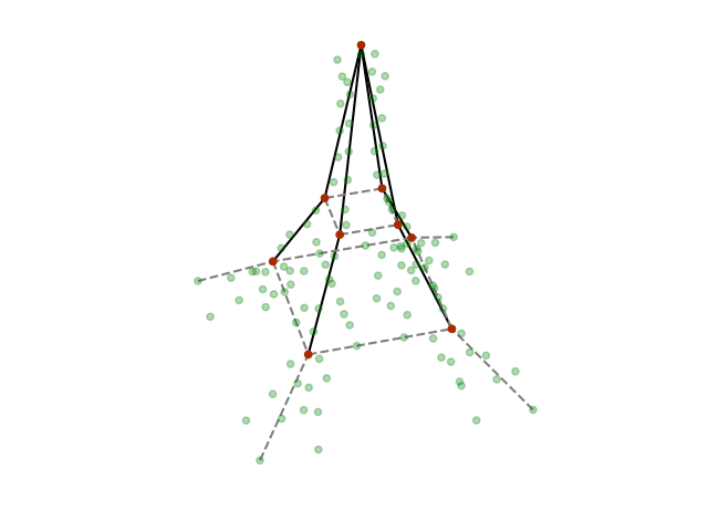
In this figure, the red dots represent the specific qubits we will use in our circuit (the green dots are not used in this demo).
The solid black lines indicate two-qubit gates between these qubits. The dashed grey lines are meant to guide the eye, but could also be used to make a more complex model by adding further two-qubit gates.
Classical data is loaded in at the bottom qubits (the “tower legs”) and the final measurement result is read out from the top “peak” qubit. The order of gate execution proceeds vertically from bottom to top, and clockwise at each level.
The code below creates this particular quantum circuit configuration in PennyLane:
peak_qubit = 8

def controlled_rotation(phi, wires):
    qml.RY(phi, wires=wires[1])
    qml.CNOT(wires=wires)
    qml.RY(-phi, wires=wires[1])
    qml.CNOT(wires=wires)

@qml.qnode(dev, interface="tf")
def circuit(weights, data):

    # Input classical data loaded into qubits at second level
    for idx in range(4):
        if data[idx]:
            qml.PauliX(wires=idx)

    # Interact qubits from second and third levels
    for idx in range(4):
        qml.CNOT(wires=[idx, idx + 4])

    # Interact qubits from third level with peak using parameterized gates
    for idx, wire in enumerate(range(4, 8)):
        controlled_rotation(weights[idx], wires=[wire, peak_qubit])

    return qml.expval(qml.PauliZ(wires=peak_qubit))
Training the circuit
Let’s now leverage this variational circuit to tackle a toy classification problem. For the purposes of this demo, we will consider a very simple classifier:
if the first input qubit is in the state \(\mid 0 \rangle\), the model should make the prediction “0”, and
if the first input qubit is in the state \(\mid 1 \rangle\), the model should predict “1” (independent of the states of all other qubits).
In other words, the idealized trained model should learn an identity transformation between the first qubit and the final one, while ignoring the states of all other qubits.
With this goal in mind, we can create a basic cost function. This cost function randomly samples possible 4-bit input bitstrings, and compares the circuit’s output with the value of the first bit. The other bits can be thought of as noise that we don’t want our model to learn.
import tensorflow as tf
np.random.seed(143)
init_weights = np.pi * np.random.rand(4)

weights = tf.Variable(init_weights, dtype=tf.float64)

data = np.random.randint(0, 2, size=4)

def cost():
    data = np.random.randint(0, 2, size=4)
    label = data[0]
    output = (-circuit(weights, data) + 1) / 2
    return tf.abs(output - label) ** 2

opt = tf.keras.optimizers.Adam(learning_rate=0.1)

for step in range(100):
    opt.minimize(cost, weights)
    if step % 5 == 0:
        print("Step {}: cost={}".format(step, cost()))

print("Final cost value: {}".format(cost()))
Out:
Step 0: cost=0.00016714805870154947
Step 5: cost=0.996033675363325
Step 10: cost=0.6155194682134244
Step 15: cost=0.999094333759448
Step 20: cost=0.005043049850429249
Step 25: cost=0.8981007649191639
Step 30: cost=0.6573246599021019
Step 35: cost=8.465054293083085e-07
Step 40: cost=0.6788142780522586
Step 45: cost=0.3556685123234262
Step 50: cost=0.026910206671360015
Step 55: cost=0.08898491577262835
Step 60: cost=0.31026489878494545
Step 65: cost=0.02024610375919167
Step 70: cost=0.007934105929226831
Step 75: cost=0.0005895204131158849
Step 80: cost=0.0005427646474345238
Step 85: cost=8.379720526363599e-07
Step 90: cost=5.347187868043335e-05
Step 95: cost=8.521633398927975e-07
Final cost value: 1.044140829353779e-05
Success! The circuit has learned to transfer the state of the first qubit to the state of the last qubit, while ignoring the state of all other input qubits.
The programmable three-dimensional configurations of neutral-atom quantum computers provide a special tool that is hard to replicate in other platforms. Could the physical arrangement of qubits, in particular the third dimension, be leveraged to make quantum algorithms more sparse or efficient? Could neutral-atom systems—with their unique programmability of the geometry—allow us to rapidly prototype and experiment with new circuit topologies? What possibilities could this open up for quantum computing, quantum chemistry, or quantum machine learning?
References
- 1
Daniel Barredo, Vincent Lienhard, Sylvain de Leseleuc, Thierry Lahaye, and Antoine Browaeys. “Synthetic three-dimensional atomic structures assembled atom by atom.” arXiv:1712.02727, 2017.