Note
Click here to download the full example code
Quantum models as Fourier series
Authors: Maria Schuld and Johannes Jakob Meyer — Posted: 24 August 2020. Last updated: 15 January 2021.
This demonstration is based on the paper The effect of data encoding on the expressive power of variational quantum machine learning models by Schuld, Sweke, and Meyer (2020) 1.
The paper links common quantum machine learning models designed for near-term quantum computers to Fourier series (and, in more general, to Fourier-type sums). With this link, the class of functions a quantum model can learn (i.e., its “expressivity”) can be characterized by the model’s control of the Fourier series’ frequencies and coefficients.
Background
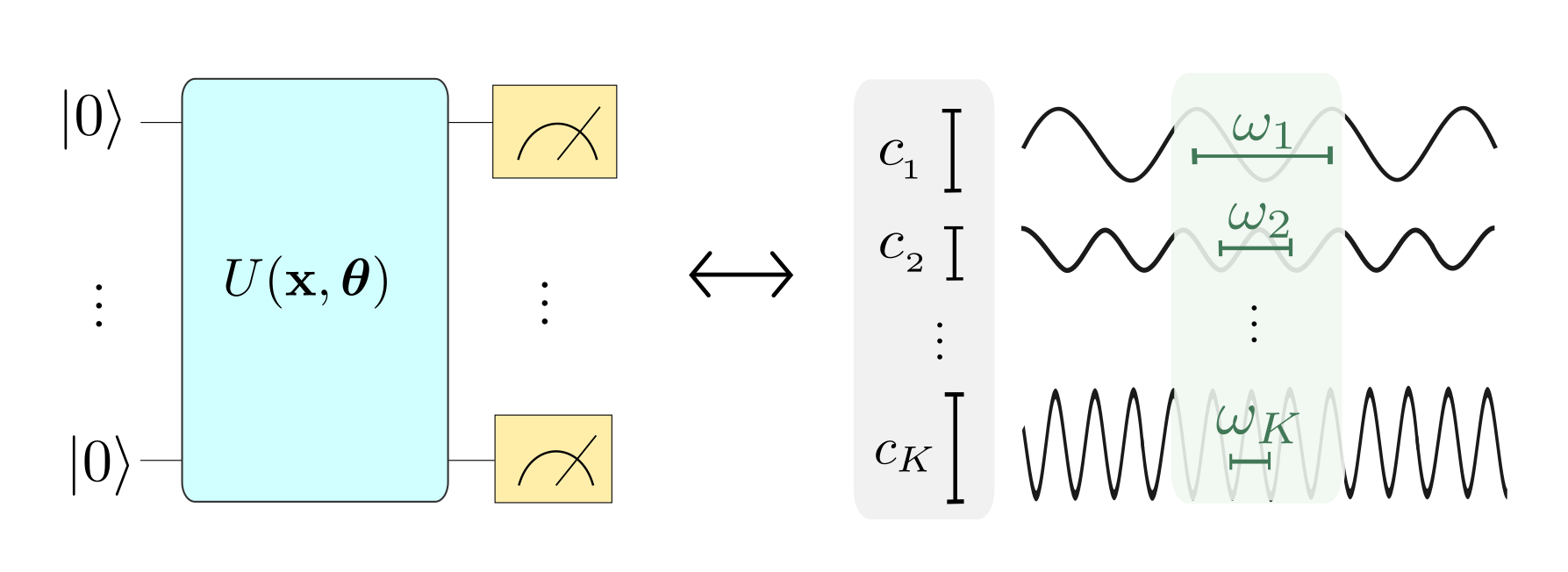
Ref. 1 considers quantum machine learning models of the form
where \(M\) is a measurement observable and \(U(x, \boldsymbol \theta)\) is a variational quantum circuit that encodes a data input \(x\) and depends on a set of parameters \(\boldsymbol \theta\). Here we will restrict ourselves to one-dimensional data inputs, but the paper motivates that higher-dimensional features simply generalize to multi-dimensional Fourier series.
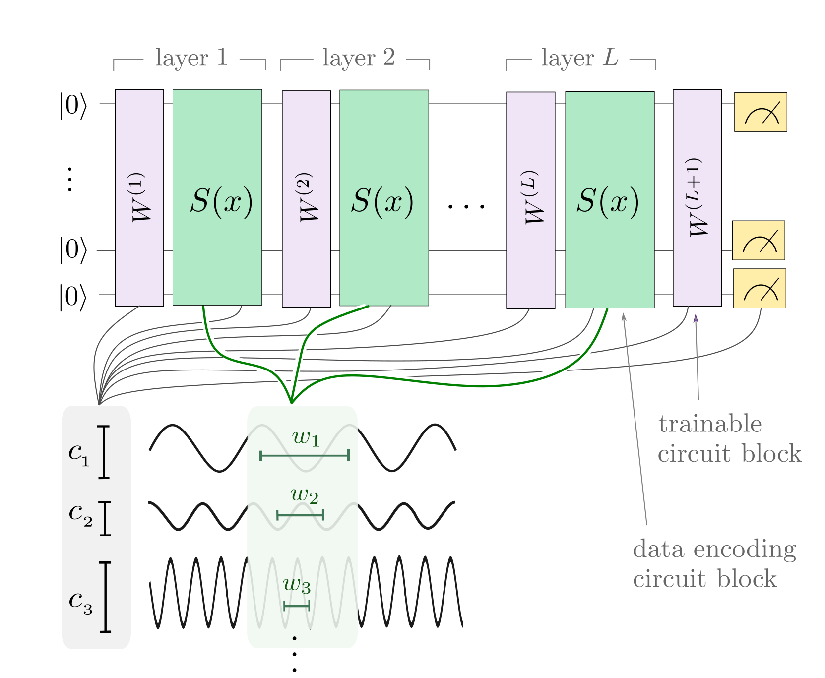
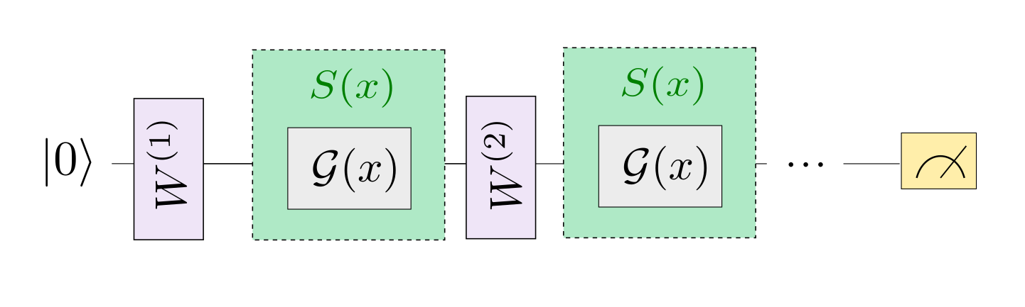
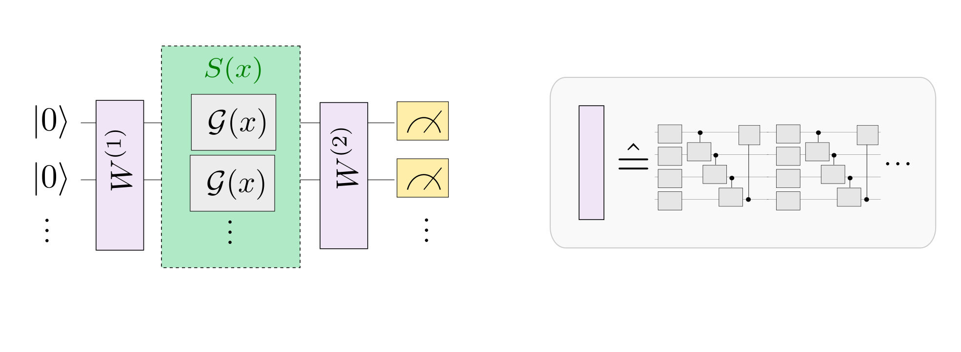
The circuit itself repeats \(L\) layers, each consisting of a data-encoding circuit block \(S(x)\) and a trainable circuit block \(W(\boldsymbol \theta)\) that is controlled by the parameters \(\boldsymbol \theta\). The data encoding block consists of gates of the form \(\mathcal{G}(x) = e^{-ix H}\), where \(H\) is a Hamiltonian. A prominent example of such gates are Pauli rotations.
The paper shows how such a quantum model can be written as a Fourier-type sum of the form
As illustrated in the picture below (which is Figure 1 from the paper), the “encoding Hamiltonians” in \(S(x)\) determine the set \(\Omega\) of available “frequencies”, and the remainder of the circuit, including the trainable parameters, determines the coefficients \(c_{\omega}\).
The paper demonstrates many of its findings for circuits in which \(\mathcal{G}(x)\) is a single-qubit Pauli rotation gate. For example, it shows that \(r\) repetitions of a Pauli rotation-encoding gate in “sequence” (on the same qubit, but with multiple layers \(r=L\)) or in “parallel” (on \(r\) different qubits, with \(L=1\)) creates a quantum model that can be expressed as a Fourier series of the form
where \(\Omega = \{ -r, \dots, -1, 0, 1, \dots, r\}\) is a spectrum of consecutive integer-valued frequencies up to degree \(r\).
As a result, we expect quantum models that encode an input \(x\) by \(r\) Pauli rotations to only be able to fit Fourier series of at most degree \(r\).
Goal of this demonstration
The experiments below investigate this “Fourier-series”-like nature of quantum models by showing how to reproduce the simulations underlying Figures 3, 4 and 5 in Section II of the paper:
Figures 3 and 4 are function-fitting experiments, where quantum models with different encoding strategies have the task to fit Fourier series up to a certain degree. As in the paper, we will use examples of qubit-based quantum circuits where a single data feature is encoded via Pauli rotations.
Figure 5 plots the Fourier coefficients of randomly sampled instances from a family of quantum models which is defined by some parametrized ansatz.
The code is presented so you can easily modify it in order to play around with other settings and models. The settings used in the paper are given in the various subsections.
First of all, let’s make some imports and define a standard loss function for the training.
import matplotlib.pyplot as plt
import pennylane as qml
from pennylane import numpy as np

np.random.seed(42)

def square_loss(targets, predictions):
    loss = 0
    for t, p in zip(targets, predictions):
        loss += (t - p) ** 2
    loss = loss / len(targets)
    return 0.5*loss
Part I: Fitting Fourier series with serial Pauli-rotation encoding
First we will reproduce Figures 3 and 4 from the paper. These show how quantum models that use Pauli rotations as data-encoding gates can only fit Fourier series up to a certain degree. The degree corresponds to the number of times that the Pauli gate gets repeated in the quantum model.
Let us consider circuits where the encoding gate gets repeated sequentially (as in Figure 2a of the paper). For simplicity we will only look at single-qubit circuits:
Define a target function
We first define a (classical) target function which will be used as a “ground truth” that the quantum model has to fit. The target function is constructed as a Fourier series of a specific degree.
We also allow for a rescaling of the data by a hyperparameter scaling,
which we will do in the quantum model as well. As shown in 1, for the quantum model to
learn the classical model in the experiment below,
the scaling of the quantum model and the target function have to match,
which is an important observation for
the design of quantum machine learning models.
degree = 1  # degree of the target function
scaling = 1  # scaling of the data
coeffs = [0.15 + 0.15j]*degree  # coefficients of non-zero frequencies
coeff0 = 0.1  # coefficient of zero frequency

def target_function(x):
    """Generate a truncated Fourier series, where the data gets re-scaled."""
    res = coeff0
    for idx, coeff in enumerate(coeffs):
        exponent = np.complex128(scaling * (idx+1) * x * 1j)
        conj_coeff = np.conjugate(coeff)
        res += coeff * np.exp(exponent) + conj_coeff * np.exp(-exponent)
    return np.real(res)
Let’s have a look at it.
Note
To reproduce the figures in the paper, you can use the following settings in the cells above:
For the settings
degree = 1
coeffs = (0.15 + 0.15j) * degree
coeff0 = 0.1
this function is the ground truth \(g(x) = \sum_{n=-1}^1 c_{n} e^{-nix}\) from Figure 3 in the paper.
To get the ground truth \(g'(x) = \sum_{n=-2}^2 c_{n} e^{-nix}\) with \(c_0=0.1\), \(c_1 = c_2 = 0.15 - 0.15i\) from Figure 3, you need to increase the degree to two:
degree = 2
The ground truth from Figure 4 can be reproduced by changing the settings to:
degree = 5
coeffs = (0.05 + 0.05j) * degree
coeff0 = 0.0
Define the serial quantum model
We now define the quantum model itself.
scaling = 1

dev = qml.device('default.qubit', wires=1)

def S(x):
    """Data-encoding circuit block."""
    qml.RX(scaling * x, wires=0)

def W(theta):
    """Trainable circuit block."""
    qml.Rot(theta[0], theta[1], theta[2], wires=0)


@qml.qnode(dev, interface="autograd")
def serial_quantum_model(weights, x):

    for theta in weights[:-1]:
        W(theta)
        S(x)

    # (L+1)'th unitary
    W(weights[-1])

    return qml.expval(qml.PauliZ(wires=0))
You can run the following cell multiple times, each time sampling different weights, and therefore different quantum models.
r = 1 # number of times the encoding gets repeated (here equal to the number of layers)
weights = 2 * np.pi * np.random.random(size=(r+1, 3), requires_grad=True) # some random initial weights
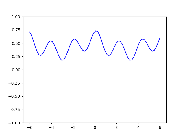
x = np.linspace(-6, 6, 70, requires_grad=False)
random_quantum_model_y = [serial_quantum_model(weights, x_) for x_ in x]
plt.plot(x, random_quantum_model_y, c='blue')
plt.ylim(-1,1)
plt.show()
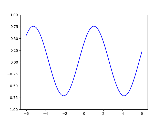
No matter what weights are picked, the single qubit model for L=1 will always be a sine function of a fixed frequency. The weights merely influence the amplitude, y-shift, and phase of the sine.
This observation is formally derived in Section II.A of the paper.
Note
You can increase the number of layers. Figure 4 from the paper, for
example, uses the settings L=1, L=3 and L=5.
Finally, let’s look at the circuit we just created:
print(qml.draw(serial_quantum_model)(weights, x[-1]))
Out:
0: ──Rot(2.35,5.97,4.60)──RX(6.00)──Rot(3.76,0.98,0.98)─┤ <Z>
Fit the model to the target
The next step is to optimize the weights in order to fit the ground truth.
def cost(weights, x, y):
    predictions = [serial_quantum_model(weights, x_) for x_ in x]
    return square_loss(y, predictions)

max_steps = 50
opt = qml.AdamOptimizer(0.3)
batch_size = 25
cst = [cost(weights, x, target_y)]  # initial cost

for step in range(max_steps):

    # Select batch of data
    batch_index = np.random.randint(0, len(x), (batch_size,))
    x_batch = x[batch_index]
    y_batch = target_y[batch_index]

    # Update the weights by one optimizer step
    weights, _, _ = opt.step(cost, weights, x_batch, y_batch)

    # Save, and possibly print, the current cost
    c = cost(weights, x, target_y)
    cst.append(c)
    if (step + 1) % 10 == 0:
        print("Cost at step {0:3}: {1}".format(step + 1, c))
Out:
Cost at step  10: 0.03212041720004578
Cost at step  20: 0.013853561883024685
Cost at step  30: 0.004049396436389444
Cost at step  40: 0.0005624933894468351
Cost at step  50: 8.145777333271227e-05
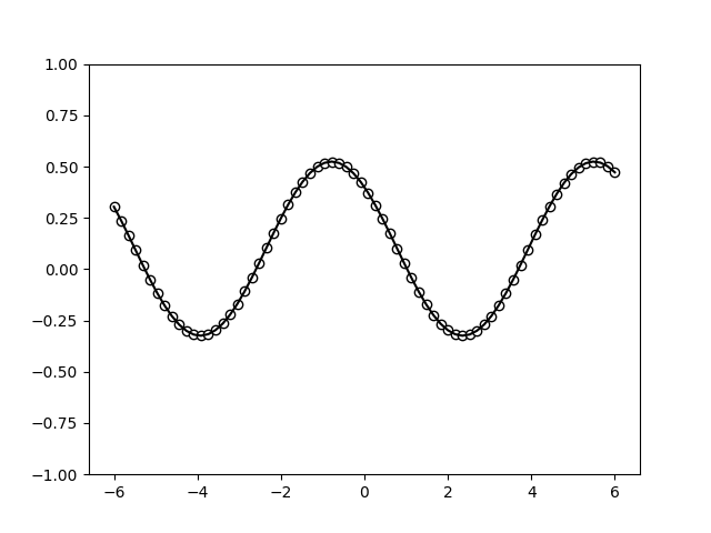
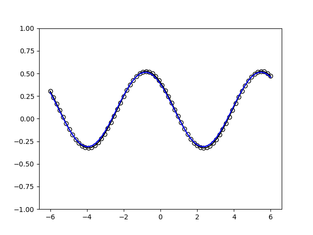
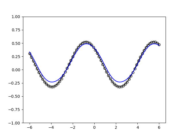
To continue training, you may just run the above cell again. Once you are happy, you can use the trained model to predict function values, and compare them with the ground truth.
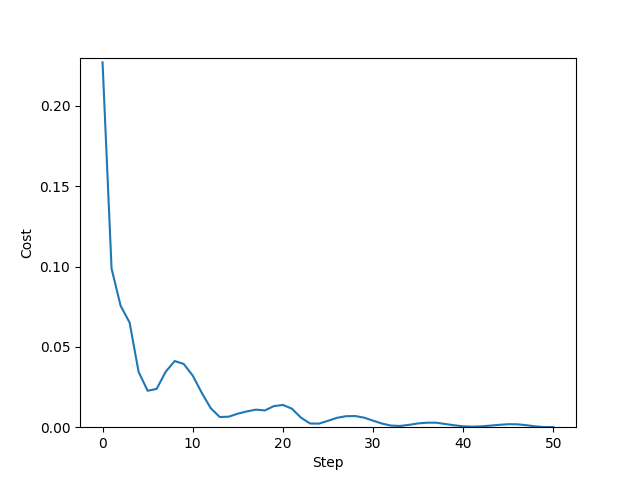
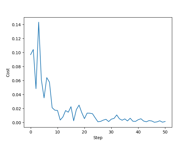
Let’s also have a look at the cost during training.
plt.plot(range(len(cst)), cst)
plt.ylabel("Cost")
plt.xlabel("Step")
plt.ylim(0, 0.23)
plt.show();
With the initial settings and enough training steps, the quantum model learns to fit the ground truth perfectly. This is expected, since the number of Pauli-rotation-encoding gates and the degree of the ground truth Fourier series are both one.
If the ground truth’s degree is larger than the number of layers in the
quantum model, the fit will look much less accurate. And finally, we
also need to have the correct scaling of the data: if one of the models
changes the scaling parameter (which effectively scales the
frequencies), fitting does not work even with enough encoding
repetitions.
Note
You will find that the training takes much longer, and needs a lot more steps to converge for larger L. Some initial weights may not even converge to a good solution at all; the training seems to get stuck in a minimum.
It is an open research question whether for asymptotically large L, the single qubit model can fit any function by constructing arbitrary Fourier coefficients.
Part II: Fitting Fourier series with parallel Pauli-rotation encoding
Our next task is to repeat the function-fitting experiment for a circuit where the Pauli rotation gate gets repeated \(r\) times on different qubits, using a single layer \(L=1\).
As shown in the paper, we expect similar results to the serial model: a Fourier series of degree \(r\) can only be fitted if there are at least \(r\) repetitions of the encoding gate in the quantum model. However, in practice this experiment is a bit harder, since the dimension of the trainable unitaries \(W\) grows quickly with the number of qubits.
In the paper, the investigations are made with the assumption that the
purple trainable blocks \(W\) are arbitrary unitaries. We could use
the ArbitraryUnitary template, but since this
template requires a number of parameters that grows exponentially with
the number of qubits (\(4^L-1\) to be precise), this quickly becomes
cumbersome to train.
We therefore follow Figure 4 in the paper and use an ansatz for \(W\).
Define the parallel quantum model
The ansatz is PennyLane’s layer structure called
StronglyEntanglingLayers, and as the name suggests, it has itself a
user-defined number of layers (which we will call “ansatz layers” to
avoid confusion).
from pennylane.templates import StronglyEntanglingLayers
Let’s have a quick look at the ansatz itself for 3 qubits by making a dummy circuit of 2 ansatz layers:
n_ansatz_layers = 2
n_qubits = 3

dev = qml.device('default.qubit', wires=4)

@qml.qnode(dev, interface="autograd")
def ansatz(weights):
    StronglyEntanglingLayers(weights, wires=range(n_qubits))
    return qml.expval(qml.Identity(wires=0))

weights_ansatz = 2 * np.pi * np.random.random(size=(n_ansatz_layers, n_qubits, 3))
print(qml.draw(ansatz, expansion_strategy="device")(weights_ansatz))
Out:
0: ──Rot(1.38,4.29,0.48)─╭●────╭X──Rot(4.26,3.55,1.68)─╭●─╭X────┤  <I>
1: ──Rot(5.35,3.11,3.02)─╰X─╭●─│───Rot(5.52,5.01,4.14)─│──╰●─╭X─┤
2: ──Rot(3.72,5.18,2.19)────╰X─╰●──Rot(5.34,5.45,4.45)─╰X────╰●─┤
Now we define the actual quantum model.
scaling = 1
r = 3

dev = qml.device('default.qubit', wires=r)

def S(x):
    """Data-encoding circuit block."""
    for w in range(r):
        qml.RX(scaling * x, wires=w)

def W(theta):
    """Trainable circuit block."""
    StronglyEntanglingLayers(theta, wires=range(r))


@qml.qnode(dev, interface="autograd")
def parallel_quantum_model(weights, x):

    W(weights[0])
    S(x)
    W(weights[1])

    return qml.expval(qml.PauliZ(wires=0))
Again, you can sample random weights and plot the model function:
trainable_block_layers = 3
weights = 2 * np.pi * np.random.random(size=(2, trainable_block_layers, r, 3), requires_grad=True)

x = np.linspace(-6, 6, 70, requires_grad=False)
random_quantum_model_y = [parallel_quantum_model(weights, x_) for x_ in x]

plt.plot(x, random_quantum_model_y, c='blue')
plt.ylim(-1,1)
plt.show();
Training the model
Training the model is done exactly as before, but it may take a lot longer this time. We set a default of 25 steps, which you should increase if necessary. Small models of <6 qubits usually converge after a few hundred steps at most—but this depends on your settings.
def cost(weights, x, y):
    predictions = [parallel_quantum_model(weights, x_) for x_ in x]
    return square_loss(y, predictions)

max_steps = 50
opt = qml.AdamOptimizer(0.3)
batch_size = 25
cst = [cost(weights, x, target_y)]  # initial cost

for step in range(max_steps):

    # select batch of data
    batch_index = np.random.randint(0, len(x), (batch_size,))
    x_batch = x[batch_index]
    y_batch = target_y[batch_index]

    # update the weights by one optimizer step
    weights, _, _ = opt.step(cost, weights, x_batch, y_batch)

    # save, and possibly print, the current cost
    c = cost(weights, x, target_y)
    cst.append(c)
    if (step + 1) % 10 == 0:
        print("Cost at step {0:3}: {1}".format(step + 1, c))
Out:
Cost at step  10: 0.017166449445318976
Cost at step  20: 0.005497199314425964
Cost at step  30: 0.004784402394898685
Cost at step  40: 0.004015481434555319
Cost at step  50: 0.0013998102989783007
plt.plot(range(len(cst)), cst)
plt.ylabel("Cost")
plt.xlabel("Step")
plt.show();
Note
To reproduce the right column in Figure 4 from the paper, use the
correct ground truth, \(r=3\) and trainable_block_layers=3,
as well as sufficiently many training steps. The amount of steps
depends on the initial weights and other hyperparameters, and
in some settings training may not converge to zero error at all.
Part III: Sampling Fourier coefficients
When we use a trainable ansatz above, it is possible that even with enough repetitions of the data-encoding Pauli rotation, the quantum model cannot fit the circuit, since the expressivity of quantum models also depends on the Fourier coefficients the model can create.
Figure 5 in 1 shows Fourier coefficients from quantum models sampled from a model family defined by an ansatz for the trainable circuit block. For this we need a function that numerically computes the Fourier coefficients of a periodic function f with period \(2 \pi\).
def fourier_coefficients(f, K):
    """
    Computes the first 2*K+1 Fourier coefficients of a 2*pi periodic function.
    """
    n_coeffs = 2 * K + 1
    t = np.linspace(0, 2 * np.pi, n_coeffs, endpoint=False)
    y = np.fft.rfft(f(t)) / t.size
    return y
Define your quantum model
Now we need to define a quantum model. This could be any model, using a
qubit or continuous-variable circuit, or one of the quantum models from
above. We will use a slight derivation of the parallel_qubit_model()
from above, this time using the BasicEntanglerLayers ansatz:
from pennylane.templates import BasicEntanglerLayers

scaling = 1
n_qubits = 4

dev = qml.device('default.qubit', wires=n_qubits)

def S(x):
    """Data encoding circuit block."""
    for w in range(n_qubits):
        qml.RX(scaling * x, wires=w)

def W(theta):
    """Trainable circuit block."""
    BasicEntanglerLayers(theta, wires=range(n_qubits))


@qml.qnode(dev, interface="autograd")
def quantum_model(weights, x):

    W(weights[0])
    S(x)
    W(weights[1])

    return qml.expval(qml.PauliZ(wires=0))
It will also be handy to define a function that samples different random weights of the correct size for the model.
n_ansatz_layers = 1

def random_weights():
    return 2 * np.pi * np.random.random(size=(2, n_ansatz_layers, n_qubits))
Now we can compute the first few Fourier coefficients for samples from
this model. The samples are created by randomly sampling different
parameters using the random_weights() function.
n_coeffs = 5
n_samples = 100


coeffs = []
for i in range(n_samples):

    weights = random_weights()

    def f(x):
        return np.array([quantum_model(weights, x_) for x_ in x])

    coeffs_sample = fourier_coefficients(f, n_coeffs)
    coeffs.append(coeffs_sample)

coeffs = np.array(coeffs)
coeffs_real = np.real(coeffs)
coeffs_imag = np.imag(coeffs)
Let’s plot the real vs. the imaginary part of the coefficients. As a sanity check, the \(c_0\) coefficient should be real, and therefore have no contribution on the y-axis.
n_coeffs = len(coeffs_real[0])

fig, ax = plt.subplots(1, n_coeffs, figsize=(15, 4))

for idx, ax_ in enumerate(ax):
    ax_.set_title(r"$c_{}$".format(idx))
    ax_.scatter(coeffs_real[:, idx], coeffs_imag[:, idx], s=20,
                facecolor='white', edgecolor='red')
    ax_.set_aspect("equal")
    ax_.set_ylim(-1, 1)
    ax_.set_xlim(-1, 1)


plt.tight_layout(pad=0.5)
plt.show();
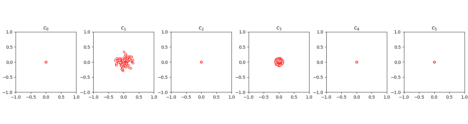
Playing around with different quantum models, you will find
that some quantum models create different distributions over
the coefficients than others. For example BasicEntanglingLayers
(with the default Pauli-X rotation) seems to have a structure
that forces the even Fourier coefficients to zero, while
StronglyEntanglingLayers will have a non-zero variance
for all supported coefficients.
Note also how the variance of the distribution decreases for growing orders of the coefficients—an effect linked to the convergence of a Fourier series.
Note
To reproduce the results from Figure 5 you have to change the ansatz (no
unitary, BasicEntanglerLayers or StronglyEntanglingLayers, and
set n_ansatz_layers either to \(1\) or \(5\)). The
StronglyEntanglingLayers requires weights of shape
size=(2, n_ansatz_layers, n_qubits, 3).
Continuous-variable model
Ref. 1 mentions that a phase rotation in continuous-variable quantum computing has a spectrum that supports all Fourier frequecies. To play with this model, we finally show you the code for a continuous-variable circuit. For example, to see its Fourier coefficients run the cell below, and then re-run the two cells above.
var = 2
n_ansatz_layers = 1
dev_cv = qml.device('default.gaussian', wires=1)

def S(x):
    qml.Rotation(x, wires=0)

def W(theta):
    """Trainable circuit block."""
    for r_ in range(n_ansatz_layers):
        qml.Displacement(theta[0], theta[1], wires=0)
        qml.Squeezing(theta[2], theta[3], wires=0)

@qml.qnode(dev_cv)
def quantum_model(weights, x):
    W(weights[0])
    S(x)
    W(weights[1])
    return qml.expval(qml.X(wires=0))

def random_weights():
    return np.random.normal(size=(2, 5 * n_ansatz_layers), loc=0, scale=var)
Note
To find out what effect so-called “non-Gaussian” gates like the
Kerr gate have, you need to install the
strawberryfields plugin
and change the device to
dev_cv = qml.device('strawberryfields.fock', wires=1, cutoff_dim=50)
References
About the authors

Maria Schuld
Johannes Jakob Meyer
Total running time of the script: ( 3 minutes 21.737 seconds)