Training and evaluating quantum kernels

Authors: Peter-Jan Derks, Paul K. Faehrmann, Elies Gil-Fuster, Tom Hubregtsen, Johannes Jakob Meyer and David Wierichs — Posted: 24 June 2021. Last updated: 18 November 2021.

Kernel methods are one of the cornerstones of classical machine learning. Here we are concerned with kernels that can be evaluated on quantum computers, quantum kernels for short. In this tutorial you will learn how to evaluate kernels, use them for classification and train them with gradient-based optimization, and all that using the functionality of PennyLane’s kernels module. The demo is based on Ref. 1, a project from Xanadu’s own QHack hackathon.

What are kernel methods?

To understand what a kernel method does, let’s first revisit one of the simplest methods to assign binary labels to datapoints: linear classification.

Imagine we want to discern two different classes of points that lie in different corners of the plane. A linear classifier corresponds to drawing a line and assigning different labels to the regions on opposing sides of the line:

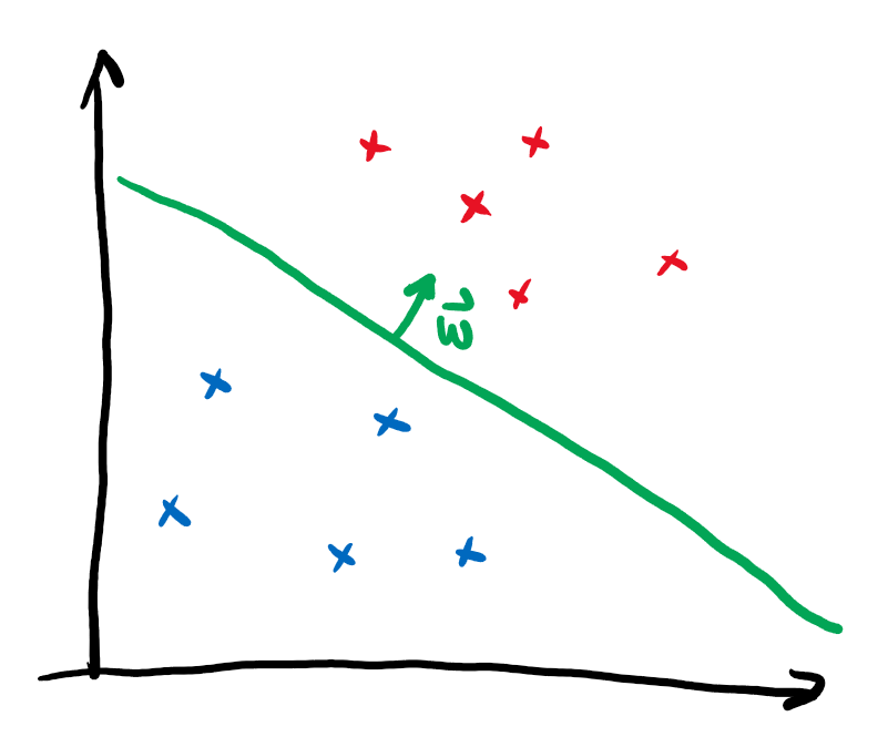
We can mathematically formalize this by assigning the label \(y\) via

\[y(\boldsymbol{x}) = \operatorname{sgn}(\langle \boldsymbol{w}, \boldsymbol{x}\rangle + b).\]

The vector \(\boldsymbol{w}\) points perpendicular to the line and thus determine its slope. The independent term \(b\) specifies the position on the plane. In this form, linear classification can also be extended to higher dimensional vectors \(\boldsymbol{x}\), where a line does not divide the entire space into two regions anymore. Instead one needs a hyperplane. It is immediately clear that this method is not very powerful, as datasets that are not separable by a hyperplane can’t be classified without error.

We can actually sneak around this limitation by performing a neat trick: if we define some map \(\phi(\boldsymbol{x})\) that embeds our datapoints into a larger feature space and then perform linear classification there, we could actually realise non-linear classification in our original space!

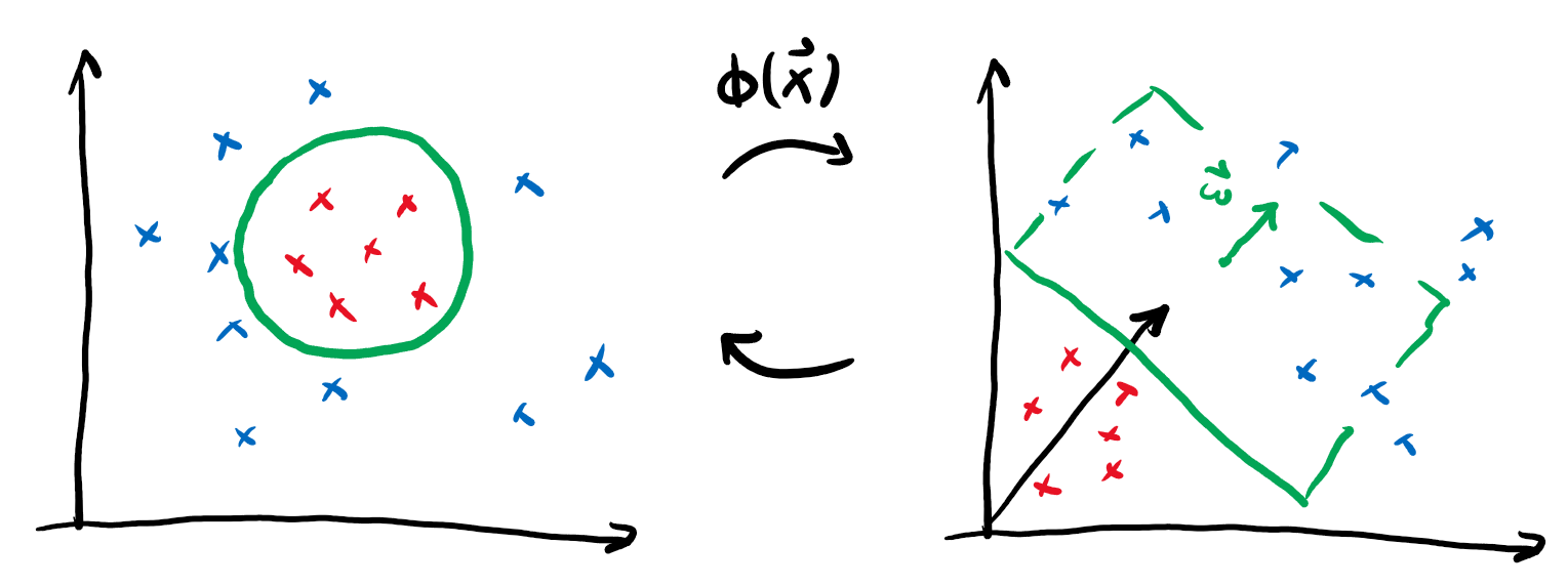
If we go back to the expression for our prediction and include the embedding, we get

\[y(\boldsymbol{x}) = \operatorname{sgn}(\langle \boldsymbol{w}, \phi(\boldsymbol{x})\rangle + b).\]

We will forgo one tiny step, but it can be shown that for the purpose of optimal classification, we can choose the vector defining the decision boundary as a linear combination of the embedded datapoints \(\boldsymbol{w} = \sum_i \alpha_i \phi(\boldsymbol{x}_i)\). Putting this into the formula yields

\[y(\boldsymbol{x}) = \operatorname{sgn}\left(\sum_i \alpha_i \langle \phi(\boldsymbol{x}_i), \phi(\boldsymbol{x})\rangle + b\right).\]

This rewriting might not seem useful at first, but notice the above formula only contains inner products between vectors in the embedding space:

\[k(\boldsymbol{x}_i, \boldsymbol{x}_j) = \langle \phi(\boldsymbol{x}_i), \phi(\boldsymbol{x}_j)\rangle.\]

We call this function the kernel. It provides the advantage that we can often find an explicit formula for the kernel \(k\) that makes it superfluous to actually perform the (potentially expensive) embedding \(\phi\). Consider for example the following embedding and the associated kernel:

\[\begin{split}\phi((x_1, x_2)) &= (x_1^2, \sqrt{2} x_1 x_2, x_2^2) \\ k(\boldsymbol{x}, \boldsymbol{y}) &= x_1^2 y_1^2 + 2 x_1 x_2 y_1 y_2 + x_2^2 y_2^2 = \langle \boldsymbol{x}, \boldsymbol{y} \rangle^2.\end{split}\]

This means by just replacing the regular scalar product in our linear classification with the map \(k\), we can actually express much more intricate decision boundaries!

This is very important, because in many interesting cases the embedding \(\phi\) will be much costlier to compute than the kernel \(k\).

In this demo, we will explore one particular kind of kernel that can be realized on near-term quantum computers, namely Quantum Embedding Kernels (QEKs). These are kernels that arise from embedding data into the space of quantum states. We formalize this by considering a parameterised quantum circuit \(U(\boldsymbol{x})\) that maps a datapoint \(\boldsymbol{x}\) to the state

\[|\psi(\boldsymbol{x})\rangle = U(\boldsymbol{x}) |0 \rangle.\]

The kernel value is then given by the overlap of the associated embedded quantum states

\[k(\boldsymbol{x}_i, \boldsymbol{x}_j) = | \langle\psi(\boldsymbol{x}_i)|\psi(\boldsymbol{x}_j)\rangle|^2.\]

A toy problem

In this demo, we will treat a toy problem that showcases the inner workings of classification with quantum embedding kernels, training variational embedding kernels and the available functionalities to do both in PennyLane. We of course need to start with some imports:

from pennylane import numpy as np
import matplotlib as mpl

np.random.seed(1359)

And we proceed right away to create a dataset to work with, the DoubleCake dataset. Firstly, we define two functions to enable us to generate the data. The details of these functions are not essential for understanding the demo, so don’t mind them if they are confusing.

def _make_circular_data(num_sectors):
    """Generate datapoints arranged in an even circle."""
    center_indices = np.array(range(0, num_sectors))
    sector_angle = 2 * np.pi / num_sectors
    angles = (center_indices + 0.5) * sector_angle
    x = 0.7 * np.cos(angles)
    y = 0.7 * np.sin(angles)
    labels = 2 * np.remainder(np.floor_divide(angles, sector_angle), 2) - 1

    return x, y, labels


def make_double_cake_data(num_sectors):
    x1, y1, labels1 = _make_circular_data(num_sectors)
    x2, y2, labels2 = _make_circular_data(num_sectors)

    # x and y coordinates of the datapoints
    x = np.hstack([x1, 0.5 * x2])
    y = np.hstack([y1, 0.5 * y2])

    # Canonical form of dataset
    X = np.vstack([x, y]).T

    labels = np.hstack([labels1, -1 * labels2])

    # Canonical form of labels
    Y = labels.astype(int)

    return X, Y

Next, we define a function to help plot the DoubleCake data:

def plot_double_cake_data(X, Y, ax, num_sectors=None):
    """Plot double cake data and corresponding sectors."""
    x, y = X.T
    cmap = mpl.colors.ListedColormap(["#FF0000", "#0000FF"])
    ax.scatter(x, y, c=Y, cmap=cmap, s=25, marker="s")

    if num_sectors is not None:
        sector_angle = 360 / num_sectors
        for i in range(num_sectors):
            color = ["#FF0000", "#0000FF"][(i % 2)]
            other_color = ["#FF0000", "#0000FF"][((i + 1) % 2)]
            ax.add_artist(
                mpl.patches.Wedge(
                    (0, 0),
                    1,
                    i * sector_angle,
                    (i + 1) * sector_angle,
                    lw=0,
                    color=color,
                    alpha=0.1,
                    width=0.5,
                )
            )
            ax.add_artist(
                mpl.patches.Wedge(
                    (0, 0),
                    0.5,
                    i * sector_angle,
                    (i + 1) * sector_angle,
                    lw=0,
                    color=other_color,
                    alpha=0.1,
                )
            )
            ax.set_xlim(-1, 1)

    ax.set_ylim(-1, 1)
    ax.set_aspect("equal")
    ax.axis("off")

    return ax

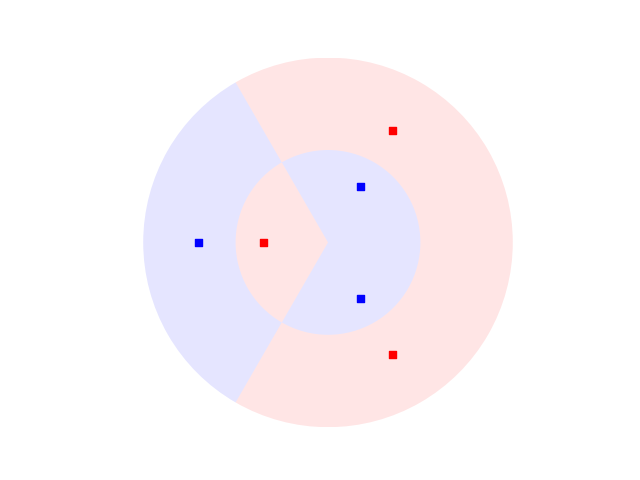
Let’s now have a look at our dataset. In our example, we will work with 3 sectors:

import matplotlib.pyplot as plt

num_sectors = 3
X, Y = make_double_cake_data(num_sectors)

ax = plot_double_cake_data(X, Y, plt.gca(), num_sectors=num_sectors)

Defining a Quantum Embedding Kernel

PennyLane’s kernels module allows for a particularly simple implementation of Quantum Embedding Kernels. The first ingredient we need for this is an ansatz, which we will construct by repeating a layer as building block. Let’s start by defining this layer:

import pennylane as qml


def layer(x, params, wires, i0=0, inc=1):
    """Building block of the embedding ansatz"""
    i = i0
    for j, wire in enumerate(wires):
        qml.Hadamard(wires=[wire])
        qml.RZ(x[i % len(x)], wires=[wire])
        i += inc
        qml.RY(params[0, j], wires=[wire])

    qml.broadcast(unitary=qml.CRZ, pattern="ring", wires=wires, parameters=params[1])

To construct the ansatz, this layer is repeated multiple times, reusing the datapoint x but feeding different variational parameters params into each of them. Together, the datapoint and the variational parameters fully determine the embedding ansatz \(U(\boldsymbol{x})\). In order to construct the full kernel circuit, we also require its adjoint \(U(\boldsymbol{x})^\dagger\), which we can obtain via qml.adjoint.

def ansatz(x, params, wires):
    """The embedding ansatz"""
    for j, layer_params in enumerate(params):
        layer(x, layer_params, wires, i0=j * len(wires))


adjoint_ansatz = qml.adjoint(ansatz)


def random_params(num_wires, num_layers):
    """Generate random variational parameters in the shape for the ansatz."""
    return np.random.uniform(0, 2 * np.pi, (num_layers, 2, num_wires), requires_grad=True)

Together with the ansatz we only need a device to run the quantum circuit on. For the purpose of this tutorial we will use PennyLane’s default.qubit device with 5 wires in analytic mode.

dev = qml.device("default.qubit", wires=5, shots=None)
wires = dev.wires.tolist()

Let us now define the quantum circuit that realizes the kernel. We will compute the overlap of the quantum states by first applying the embedding of the first datapoint and then the adjoint of the embedding of the second datapoint. We finally extract the probabilities of observing each basis state.

@qml.qnode(dev, interface="autograd")
def kernel_circuit(x1, x2, params):
    ansatz(x1, params, wires=wires)
    adjoint_ansatz(x2, params, wires=wires)
    return qml.probs(wires=wires)

The kernel function itself is now obtained by looking at the probability of observing the all-zero state at the end of the kernel circuit – because of the ordering in qml.probs, this is the first entry:

def kernel(x1, x2, params):
    return kernel_circuit(x1, x2, params)[0]

Note

An alternative way to set up the kernel circuit in PennyLane would be to use the observable type Projector. This is shown in the demo on kernel-based training of quantum models, where you will also find more background information on the kernel circuit structure itself.

Before focusing on the kernel values we have to provide values for the variational parameters. At this point we fix the number of layers in the ansatz circuit to \(6\).

init_params = random_params(num_wires=5, num_layers=6)

Now we can have a look at the kernel value between the first and the second datapoint:

kernel_value = kernel(X[0], X[1], init_params)
print(f"The kernel value between the first and second datapoint is {kernel_value:.3f}")

Out:

The kernel value between the first and second datapoint is 0.093

The mutual kernel values between all elements of the dataset form the kernel matrix. We can inspect it via the qml.kernels.square_kernel_matrix method, which makes use of symmetry of the kernel, \(k(\boldsymbol{x}_i,\boldsymbol{x}_j) = k(\boldsymbol{x}_j, \boldsymbol{x}_i)\). In addition, the option assume_normalized_kernel=True ensures that we do not calculate the entries between the same datapoints, as we know them to be 1 for our noiseless simulation. Overall this means that we compute \(\frac{1}{2}(N^2-N)\) kernel values for \(N\) datapoints. To include the variational parameters, we construct a lambda function that fixes them to the values we sampled above.

init_kernel = lambda x1, x2: kernel(x1, x2, init_params)
K_init = qml.kernels.square_kernel_matrix(X, init_kernel, assume_normalized_kernel=True)

with np.printoptions(precision=3, suppress=True):
    print(K_init)

Out:

[[1.    0.093 0.012 0.721 0.149 0.055]
 [0.093 1.    0.056 0.218 0.73  0.213]
 [0.012 0.056 1.    0.032 0.191 0.648]
 [0.721 0.218 0.032 1.    0.391 0.226]
 [0.149 0.73  0.191 0.391 1.    0.509]
 [0.055 0.213 0.648 0.226 0.509 1.   ]]

Using the Quantum Embedding Kernel for predictions

The quantum kernel alone can not be used to make predictions on a dataset, becaues it is essentially just a tool to measure the similarity between two datapoints. To perform an actual prediction we will make use of scikit-learn’s Support Vector Classifier (SVC).

from sklearn.svm import SVC

To construct the SVM, we need to supply sklearn.svm.SVC with a function that takes two sets of datapoints and returns the associated kernel matrix. We can make use of the function qml.kernels.kernel_matrix that provides this functionality. It expects the kernel to not have additional parameters besides the datapoints, which is why we again supply the variational parameters via the lambda function from above. Once we have this, we can let scikit-learn adjust the SVM from our Quantum Embedding Kernel.

Note

This step does not modify the variational parameters in our circuit ansatz. What it does is solving a different optimization task for the \(\alpha\) and \(b\) vectors we introduced in the beginning.

svm = SVC(kernel=lambda X1, X2: qml.kernels.kernel_matrix(X1, X2, init_kernel)).fit(X, Y)

To see how well our classifier performs we will measure which percentage of the dataset it classifies correctly.

def accuracy(classifier, X, Y_target):
    return 1 - np.count_nonzero(classifier.predict(X) - Y_target) / len(Y_target)


accuracy_init = accuracy(svm, X, Y)
print(f"The accuracy of the kernel with random parameters is {accuracy_init:.3f}")

Out:

The accuracy of the kernel with random parameters is 0.833

We are also interested in seeing what the decision boundaries in this classification look like. This could help us spotting overfitting issues visually in more complex data sets. To this end we will introduce a second helper method.

def plot_decision_boundaries(classifier, ax, N_gridpoints=14):
    _xx, _yy = np.meshgrid(np.linspace(-1, 1, N_gridpoints), np.linspace(-1, 1, N_gridpoints))

    _zz = np.zeros_like(_xx)
    for idx in np.ndindex(*_xx.shape):
        _zz[idx] = classifier.predict(np.array([_xx[idx], _yy[idx]])[np.newaxis, :])

    plot_data = {"_xx": _xx, "_yy": _yy, "_zz": _zz}
    ax.contourf(
        _xx,
        _yy,
        _zz,
        cmap=mpl.colors.ListedColormap(["#FF0000", "#0000FF"]),
        alpha=0.2,
        levels=[-1, 0, 1],
    )
    plot_double_cake_data(X, Y, ax)

    return plot_data

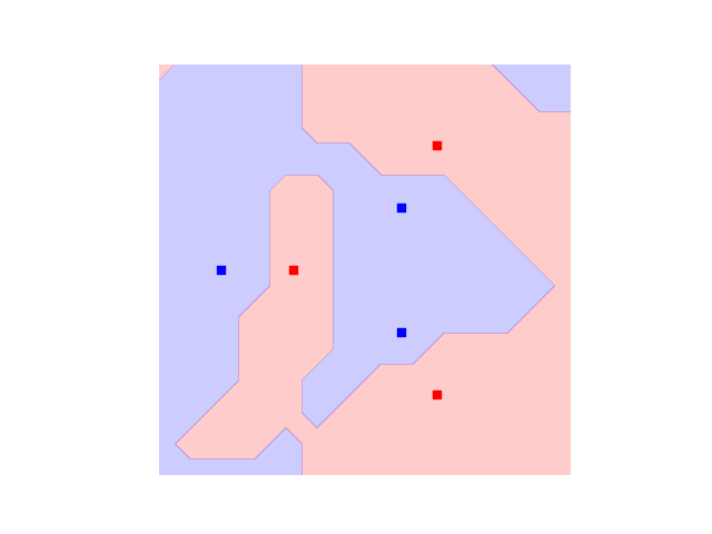
With that done, let’s have a look at the decision boundaries for our initial classifier:

init_plot_data = plot_decision_boundaries(svm, plt.gca())

We see the outer points in the dataset can be correctly classified, but we still struggle with the inner circle. But remember we have a circuit with many free parameters! It is reasonable to believe we can give values to those variational parameters which improve the overall accuracy of our SVC.

Training the Quantum Embedding Kernel

To be able to train the Quantum Embedding Kernel we need some measure of how well it fits the dataset in question. Performing an exhaustive search in parameter space is not a good solution because it is very resource intensive, and since the accuracy is a discrete quantity we would not be able to detect small improvements.

We can, however, resort to a more specialized measure, the kernel-target alignment 2. The kernel-target alignment compares the similarity predicted by the quantum kernel to the actual labels of the training data. It is based on kernel alignment, a similiarity measure between two kernels with given kernel matrices \(K_1\) and \(K_2\):

\[\operatorname{KA}(K_1, K_2) = \frac{\operatorname{Tr}(K_1 K_2)}{\sqrt{\operatorname{Tr}(K_1^2)\operatorname{Tr}(K_2^2)}}.\]

Note

Seen from a more theoretical side, \(\operatorname{KA}\) is nothing else than the cosine of the angle between the kernel matrices \(K_1\) and \(K_2\) if we see them as vectors in the space of matrices with the Hilbert-Schmidt (or Frobenius) scalar product \(\langle A, B \rangle = \operatorname{Tr}(A^T B)\). This reinforces the geometric picture of how this measure relates to objects, namely two kernels, being aligned in a vector space.

The training data enters the picture by defining an ideal kernel function that expresses the original labelling in the vector \(\boldsymbol{y}\) by assigning to two datapoints the product of the corresponding labels:

\[k_{\boldsymbol{y}}(\boldsymbol{x}_i, \boldsymbol{x}_j) = y_i y_j.\]

The assigned kernel is thus \(+1\) if both datapoints lie in the same class and \(-1\) otherwise and its kernel matrix is simply given by the outer product \(\boldsymbol{y}\boldsymbol{y}^T\). The kernel-target alignment is then defined as the kernel alignment of the kernel matrix \(K\) generated by the quantum kernel and \(\boldsymbol{y}\boldsymbol{y}^T\):

\[\operatorname{KTA}_{\boldsymbol{y}}(K) = \frac{\operatorname{Tr}(K \boldsymbol{y}\boldsymbol{y}^T)}{\sqrt{\operatorname{Tr}(K^2)\operatorname{Tr}((\boldsymbol{y}\boldsymbol{y}^T)^2)}} = \frac{\boldsymbol{y}^T K \boldsymbol{y}}{\sqrt{\operatorname{Tr}(K^2)} N}\]

where \(N\) is the number of elements in \(\boldsymbol{y}\), that is the number of datapoints in the dataset.

In summary, the kernel-target alignment effectively captures how well the kernel you chose reproduces the actual similarities of the data. It does have one drawback, however: having a high kernel-target alignment is only a necessary but not a sufficient condition for a good performance of the kernel 2. This means having good alignment is guaranteed for good performance, but optimal alignment will not always bring optimal training accuracy with it.

Let’s now come back to the actual implementation. PennyLane’s kernels module allows you to easily evaluate the kernel target alignment:

kta_init = qml.kernels.target_alignment(X, Y, init_kernel, assume_normalized_kernel=True)

print(f"The kernel-target alignment for our dataset and random parameters is {kta_init:.3f}")

Out:

The kernel-target alignment for our dataset and random parameters is 0.081

Now let’s code up an optimization loop and improve the kernel-target alignment!

We will make use of regular gradient descent optimization. To speed up the optimization we will not use the entire training set to compute \(\operatorname{KTA}\) but rather sample smaller subsets of the data at each step, we choose \(4\) datapoints at random. Remember that PennyLane’s built-in optimizer works to minimize the cost function that is given to it, which is why we have to multiply the kernel target alignment by \(-1\) to actually maximize it in the process.

Note

Currently, the function qml.kernels.target_alignment is not differentiable yet, making it unfit for gradient descent optimization. We therefore first define a differentiable version of this function.

def target_alignment(
    X,
    Y,
    kernel,
    assume_normalized_kernel=False,
    rescale_class_labels=True,
):
    """Kernel-target alignment between kernel and labels."""

    K = qml.kernels.square_kernel_matrix(
        X,
        kernel,
        assume_normalized_kernel=assume_normalized_kernel,
    )

    if rescale_class_labels:
        nplus = np.count_nonzero(np.array(Y) == 1)
        nminus = len(Y) - nplus
        _Y = np.array([y / nplus if y == 1 else y / nminus for y in Y])
    else:
        _Y = np.array(Y)

    T = np.outer(_Y, _Y)
    inner_product = np.sum(K * T)
    norm = np.sqrt(np.sum(K * K) * np.sum(T * T))
    inner_product = inner_product / norm

    return inner_product


params = init_params
opt = qml.GradientDescentOptimizer(0.2)

for i in range(500):
    # Choose subset of datapoints to compute the KTA on.
    subset = np.random.choice(list(range(len(X))), 4)
    # Define the cost function for optimization
    cost = lambda _params: -target_alignment(
        X[subset],
        Y[subset],
        lambda x1, x2: kernel(x1, x2, _params),
        assume_normalized_kernel=True,
    )
    # Optimization step
    params = opt.step(cost, params)

    # Report the alignment on the full dataset every 50 steps.
    if (i + 1) % 50 == 0:
        current_alignment = target_alignment(
            X,
            Y,
            lambda x1, x2: kernel(x1, x2, params),
            assume_normalized_kernel=True,
        )
        print(f"Step {i+1} - Alignment = {current_alignment:.3f}")

Out:

Step 50 - Alignment = 0.098
Step 100 - Alignment = 0.121
Step 150 - Alignment = 0.141
Step 200 - Alignment = 0.173
Step 250 - Alignment = 0.196
Step 300 - Alignment = 0.224
Step 350 - Alignment = 0.245
Step 400 - Alignment = 0.261
Step 450 - Alignment = 0.276
Step 500 - Alignment = 0.289

We want to assess the impact of training the parameters of the quantum kernel. Thus, let’s build a second support vector classifier with the trained kernel:

# First create a kernel with the trained parameter baked into it.
trained_kernel = lambda x1, x2: kernel(x1, x2, params)

# Second create a kernel matrix function using the trained kernel.
trained_kernel_matrix = lambda X1, X2: qml.kernels.kernel_matrix(X1, X2, trained_kernel)

# Note that SVC expects the kernel argument to be a kernel matrix function.
svm_trained = SVC(kernel=trained_kernel_matrix).fit(X, Y)

We expect to see an accuracy improvement vs. the SVM with random parameters:

accuracy_trained = accuracy(svm_trained, X, Y)
print(f"The accuracy of a kernel with trained parameters is {accuracy_trained:.3f}")

Out:

The accuracy of a kernel with trained parameters is 1.000

We have now achieved perfect classification! 🎆

Following on the results that SVM’s have proven good generalisation behavior, it will be interesting to inspect the decision boundaries of our classifier:

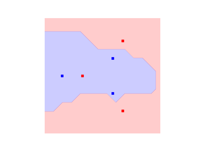
trained_plot_data = plot_decision_boundaries(svm_trained, plt.gca())

Indeed, we see that now not only every data instance falls within the correct class, but also that there are no strong artifacts that would make us distrust the model. In this sense, our approach benefits from both: on one hand it can adjust itself to the dataset, and on the other hand is not expected to suffer from bad generalisation.

References

1

Thomas Hubregtsen, David Wierichs, Elies Gil-Fuster, Peter-Jan H. S. Derks, Paul K. Faehrmann, and Johannes Jakob Meyer. “Training Quantum Embedding Kernels on Near-Term Quantum Computers.” arXiv:2105.02276, 2021.

2(1,2)

Wang, Tinghua, Dongyan Zhao, and Shengfeng Tian. “An overview of kernel alignment and its applications.” Artificial Intelligence Review 43.2: 179-192, 2015.

About the authors

Peter-Jan Derks

Peter-Jan is a PhD student in Berlin supervised by Jens Eisert. He is excited about designing near-term quantum error correction experiments and programming decoders.

Paul K. Faehrmann

Paul is a Ph.D. student in the group of Jens Eisert at the Freie Universität Berlin. His research revolves around quantum algorithms both for noisy, near-term devices and larger, fault-tolerant quantum computers

Elies Gil-Fuster

Elies is a QML researcher in Berlin interested in board games and the maths of data re-uploading PQCs. He was a Xanadu Summer Resident of the first cohort, and you can find more about him at https://eliesgilfuster.eu.

Johannes Jakob Meyer

Johannes Jakob is a PhD student in Jens Eisert's group at the FU Berlin. He strives to establish hard facts about near-term quantum devices and convert those into useful applications. His personal website is website johannesjakobmeyer.com.

David Wierichs

David is a researcher and quantum software developer at Xanadu, who likes to think about quantum gradients and how to use them in variational quantum algorithms. He enjoys sharing ideas in science and open source software and likes implementing cool stuff in PennyLane.

demos/tutorial_kernels_module

 

Download Python script

 

Download Notebook

 

View on GitHub