Intro to QSVT

Author: Juan Miguel Arrazola — Posted: May 23, 2023.

Few quantum algorithms deserve to be placed in a hall of fame: Shor’s algorithm, Grover’s algorithm, quantum phase estimation; maybe even HHL and VQE. There is now a new technique with prospects of achieving such celebrity status: the quantum singular value transformation (QSVT). Since you’re reading this, chances are you have at least heard of QSVT and its broad applicability.

This tutorial introduces the fundamental principles of QSVT with example code from PennyLane. We focus on the basics; while these techniques may appear intimidating in the literature, the fundamentals are relatively easy to grasp. Teaching you these core principles is the purpose of this tutorial.

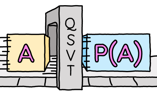
Transforming scalars encoded in matrices

My personal perspective on QSVT is that it is really a result in linear algebra that tells us how to transform matrices that are inside larger unitary matrices.

Let’s start with the simplest example: we encode a scalar \(a\) inside a 2x2 matrix \(U(a)\). By encoding we mean that the matrix depends explicitly on \(a\). This encoding can be achieved in multiple ways, for example:

\[\begin{split}U(a) = \begin{pmatrix} a & \sqrt{1-a^2}\\ \sqrt{1-a^2} & -a \end{pmatrix}.\end{split}\]

The parameter \(a\) must lie between -1 and 1 to ensure the matrix is unitary, but this is just a matter of rescaling. We want the matrix to be unitary so that it can be implemented on a quantum computer.

We now ask the crucial question that will get everything started: what happens if we repeatedly alternate multiplication of this matrix by some other matrix? 🤔 There are multiple choices for the “other matrix”, for example

\[\begin{split}S(\phi) = \begin{pmatrix} e^{i\phi} & 0\\ 0 & e^{-i\phi} \end{pmatrix},\end{split}\]

which has the advantage of being diagonal. This unitary is known as the signal-processing operator. It depends on a choice of angle \(\phi\) that will play an important role.

The answer to our question is encapsulated in a method known as quantum signal processing (QSP). If we alternate products of \(U(a)\) and \(S(\phi)\), keeping \(a\) fixed and varying \(\phi\), the top-left corner of the resulting matrix is a polynomial transformation of \(a\). Mathematically,

\[\begin{split}S(\phi_0)\prod_{k=1}^d W(a) S(\phi_k) = \begin{pmatrix} P(a) & *\\ * & * \end{pmatrix}.\end{split}\]

The asterisk \(*\) is used to indicate that we are not interested in these entries.

The intuition behind this result is that every time we multiply by \(W(a)\), its entries are transformed to a polynomial of higher degree, and by interleaving signal-processing operators, it’s possible to tune the coefficients of the polynomial. For example

\[\begin{split}S(-\pi/2) W(a) S(\pi/2) W(a) S(0) = \begin{pmatrix} 2a^2-1 & 0\\ 0 & 2a^2 -1 \end{pmatrix}.\end{split}\]

The main quantum signal processing theorem states that it is possible to find angles that implement a large class of complex polynomial transformations \(P(a)\) with maximum degree and parity determined by the number of angles 3.

The results of the theorem can then be extended to show that using additional rotations, it is possible to find \(d+1\) angles that implement any real polynomial of parity \(d \mod 2\) and maximum degree \(d\). Multiple QSP sequences can then be used to implement real polynomials of indefinite parity. Finding the desired angles can be done efficiently in practice, but identifying the best methods is an active area of research. You can learn more in our QSP demo and in Ref. 3.

For now, let’s look at a simple example of how quantum signal processing can be implemented using PennyLane. We aim to perform a transformation by the Legendre polynomial \((5 x^3 - 3x)/2\), for which we use pre-computed optimal angles. As you will soon learn, QSP can be viewed as a special case of QSVT. We thus use the qsvt() operation to construct the output matrix and compare the resulting transformation to the target polynomial.

import pennylane as qml
import numpy as np
import matplotlib.pyplot as plt


def target_poly(a):
    return 0.5 * (5 * a**3 - 3 * a)


# pre-optimized angles
angles = [-0.20409113, -0.91173829, 0.91173829, 0.20409113]


def qsvt_output(a):
    # output matrix
    out = qml.matrix(qml.qsvt(a, angles, wires=[0]))
    return out[0, 0]  # top-left entry


a_vals = np.linspace(-1, 1, 50)
qsvt = [np.real(qsvt_output(a)) for a in a_vals]  # neglect small imaginary part
target = [target_poly(a) for a in a_vals]


plt.plot(a_vals, qsvt, label="target")
plt.plot(a_vals, target, "*", label="qsvt")

plt.legend()
plt.show()

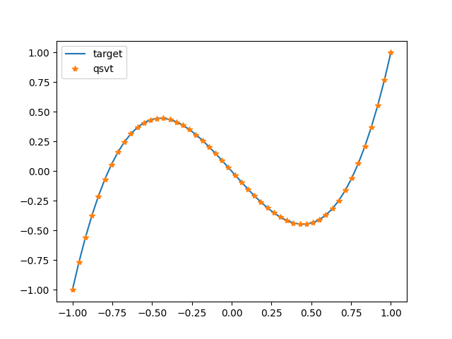
It works! 🎉 💃

Quantum signal processing is a result about multiplication of 2x2 matrices, yet it is the core principle underlying the QSVT algorithm. If you’ve made it this far, you’re in great shape for the rest to come 🥇

Transforming matrices encoded in matrices

Time to ask another key question: what if instead of encoding a scalar, we encode an entire matrix \(A\)? 🧠 This is trickier since we need to ensure that the larger operator remains unitary. A way to achieve this is to use a similar construction as in the scalar case:

\[\begin{split}U(A) = \begin{pmatrix} A & \sqrt{I-A A^\dagger}\\ \sqrt{I-A^\dagger A} & -A^\dagger \end{pmatrix}.\end{split}\]

This operator is a valid unitary regardless of the form of \(A\); it doesn’t even have to be a square matrix. We just need to ensure that \(A\) is properly normalized such that its largest singular value is bounded by 1.

Any such method of encoding a matrix inside a larger unitary is known as a block encoding. In our construction, the matrix \(A\) is encoded in the top-left block, hence the name. PennyLane supports the BlockEncode operation that follows the construction above. Let’s test it out with an example encoding first a square matrix:

# square matrix
A = [[0.1, 0.2], [0.3, 0.4]]
U1 = qml.BlockEncode(A, wires=range(2))
print("U(A):")
print(np.round(qml.matrix(U1), 2))

Out:

U(A):
[[ 0.1   0.2   0.97 -0.06]
 [ 0.3   0.4  -0.06  0.86]
 [ 0.95 -0.08 -0.1  -0.3 ]
 [-0.08  0.89 -0.2  -0.4 ]]

And also a rectangular matrix

B = [[0.5, -0.5, 0.5]]
U2 = qml.BlockEncode(B, wires=range(2))
print("U(B):")
print(np.round(qml.matrix(U2), 2))

Out:

U(B):
[[ 0.5  -0.5   0.5   0.5 ]
 [ 0.83  0.17 -0.17 -0.5 ]
 [ 0.17  0.83  0.17  0.5 ]
 [-0.17  0.17  0.83 -0.5 ]]

Notice that we haven’t really made a reference to quantum computing; everything is just linear algebra. Told you so! 😈

Quantum kicks in when we construct circuits that implement a block-encoding unitary. Arguably the hardest thing about QSVT is implementing block encodings. We don’t cover such methods in detail here, but for reference, a popular approach is to express \(A\) as a linear combination of unitaries and define associated \(\text{PREPARE}\) and \(\text{SELECT}\) operators. Then the operator

\[U=\text{PREP}^\dagger\cdot\text{SEL}\cdot\text{PREP},\]

is a block-encoding of \(A\) up to a constant factor.

Time for a third key question: Can we use the same strategy as in QSP to polynomially transform a block-encoded matrix? Because that would be fantastic 😎

For this to be possible, we need to generalize the signal-processing operator \(S(\phi)\) to higher dimensions. This can be done by using a diagonal unitary where we apply the phase \(e^{i\phi}\) to the subspace determined by the block, and the phase \(e^{-i \phi}\) everywhere else. For example, revisiting the square matrix \(A\) in the code above, where \(A\) is encoded in a two-dimensional subspace, the corresponding operator is

\[\begin{split}\begin{pmatrix} e^{i\phi} & 0 & 0 & 0\\ 0 & e^{i\phi} & 0 & 0 \\ 0 & 0 & e^{-i\phi} & 0\\ 0 & 0 & 0 & e^{-i\phi} \\ \end{pmatrix}.\end{split}\]

These are known as projector-controlled phase gates, for which we use the symbol \(\Pi(\phi)\).

When \(A\) is not square, we have to be careful and define two operators: one acting on the row subspace and another on the column subspace. Projector-controlled phase gates are implemented in PennyLane using the PCPhase operation. Here’s a simple example:

dim = 2
phi = np.pi / 2
pcp = qml.PCPhase(phi, dim, wires=range(2))
print("Pi:")
print(np.round(qml.matrix(pcp), 2))

Out:

Pi:
[[0.+1.j 0.+0.j 0.+0.j 0.+0.j]
 [0.+0.j 0.+1.j 0.+0.j 0.+0.j]
 [0.+0.j 0.+0.j 0.-1.j 0.+0.j]
 [0.+0.j 0.+0.j 0.+0.j 0.-1.j]]

As you may have guessed, this generalization of QSP does the trick. By cleverly alternating a block-encoding unitary and the appropriate projector-controlled phase gates, we can polynomially transform the encoded matrix. The result is the QSVT algorithm.

Mathematically, when the polynomial degree \(d\) is even (number of angles is \(d + 1\)), the QSVT algorithm states that

\[\begin{split}\left[\prod_{k=1}^{d/2}\Pi_{\phi_{2k-1}}U(A)^\dagger \tilde{\Pi}_{\phi_{2k}} U(A)\right]\Pi_{\phi_{d+1}}= \begin{pmatrix} P(A) & *\\ * & * \end{pmatrix}.\end{split}\]

The tilde is used in the projector-controlled phase gates to distinguish whether they act on the column or row subspaces. The polynomial transformation of \(A\) is defined in terms of its singular value decomposition

\[P(A) = \sum_k P(\sigma_k)|w_k\rangle \langle v_k|,\]

where we use braket notation to denote the left and right singular vectors. For technical reasons, the sequence looks slightly different when the polynomial degree is odd:

\[\begin{split}\tilde{\Pi}_{\phi_1}\left[\prod_{k=1}^{(d-1)/2}\Pi_{\phi_{2k}}U(A)^\dagger \tilde{\Pi}_{\phi_{2k+1}} U(A)\right]\Pi_{\phi_{d+1}}= \begin{pmatrix} P(A) & *\\ * & * \end{pmatrix}.\end{split}\]

As with QSP, it is possible to use the QSVT sequence to apply any real polynomial transformation up to degree \(d\) when using \(d+1\) angles. In fact, as long as we’re careful with conventions, we can use the same angles regardless of the dimensions of \(A\).

The QSVT construction is a beautiful result. By using a number of operations that grows linearly with the degree of the target polynomial, we can transform the singular values of arbitrary block-encoded matrices without ever having to actually perform singular value decompositions! If the block encoding circuits can be implemented in polynomial time in the number of qubits, the resulting quantum algorithm will also run in polynomial time. This is very powerful.

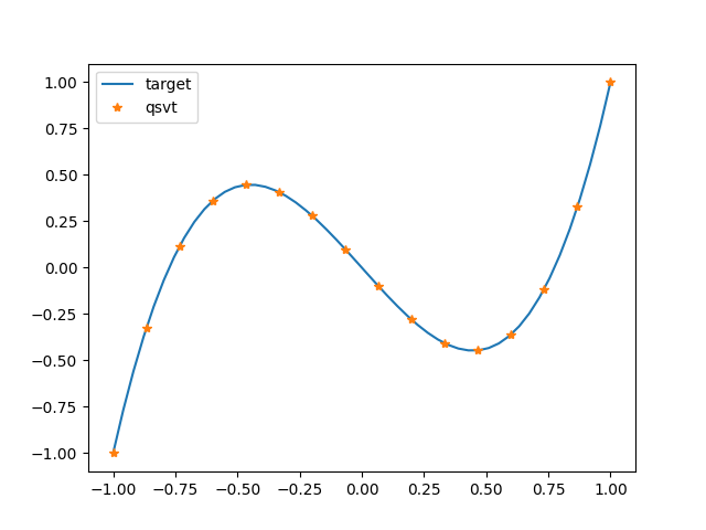
In PennyLane, implementing the QSVT transformation is as simple as using qsvt(). Let’s revisit our previous example and transform a matrix according to the same Legendre polynomial. We’ll use a diagonal matrix with eigenvalues evenly distributed between -1 and 1, allowing us to easily check the transformation.

eigvals = np.linspace(-1, 1, 16)
A = np.diag(eigvals)  # 16-dim matrix
U_A = qml.matrix(qml.qsvt)(A, angles, wires=range(5))  # block-encoded in 5-qubit system

qsvt_A = np.real(np.diagonal(U_A))[:16]  # retrieve transformed eigenvalues

plt.plot(a_vals, target, label="target")
plt.plot(eigvals, qsvt_A, "*", label="qsvt")

plt.legend()
plt.show()

The qsvt() operation is tailored for use in simulators and employs standard forms for block encodings and projector-controlled phase shifts. Advanced users can define their own version of these operators with explicit quantum circuits, and construct the resulting QSVT algorithm using the QSVT template.

Final thoughts

The original paper introducing the QSVT algorithm 1 described a series of potential applications, notably Hamiltonian simulation and solving linear systems of equations. QSVT has also been used as a unifying framework for different quantum algorithms 3. One of my favourite uses of QSVT is to transform a molecular Hamiltonian by a polynomial approximation of a step function 2. This sets large eigenvalues to zero, effectively performing a projection onto a low-energy subspace.

The PennyLane team is motivated to create tools that can empower researchers worldwide to develop the innovations that will define the present and future of quantum computing. We have designed QSVT support to help you master the concepts and perform rapid prototyping of new ideas. We look forward to seeing the innovations that will result from your journey.

References

1

András Gilyén, Yuan Su, Guang Hao Low, Nathan Wiebe, “Quantum singular value transformation and beyond: exponential improvements for quantum matrix arithmetics”, Proceedings of the 51st Annual ACM SIGACT Symposium on the Theory of Computing, 2019

2

Lin, Lin, and Yu Tong, “Near-optimal ground state preparation”, Quantum 4, 372, 2020

3(1,2,3)

John M. Martyn, Zane M. Rossi, Andrew K. Tan, and Isaac L. Chuang, “Grand Unification of Quantum Algorithms”, PRX Quantum 2, 040203, 2021

About the author

Juan Miguel Arrazola

Juan Miguel is the Algorithms Senior Team Lead at Xanadu. His work focuses on developing quantum algorithms and related software for simulating molecules and materials.

demos/tutorial_intro_qsvt

 

Download Python script

 

Download Notebook

 

View on GitHub