Compilation of quantum circuits

Author: Borja Requena — Posted: 14 June 2023.

Quantum circuits take many different forms from the moment we design them to the point where they are ready to run on a quantum device. These changes happen during the compilation process of the quantum circuits, which relies on the fact that there are many equivalent representations of quantum circuits that use different sets of gates but provide the same output.

Out of those representations, we are typically interested in finding the most suitable one for our purposes. For example, we usually look for the one that will incur the least amount of errors in the specific hardware on which we are compiling the circuit. This usually implies decomposing the quantum gates in terms of the native ones of the quantum device, adapting the operations to the hardrware’s topology, combining them to reduce the circuit depth, etc.

A crucial part of the compilation process consists of repeatedly performing minor circuit modifications. In PennyLane, we can apply transforms to our quantum functions in order to obtain equivalent ones that may be more convenient for our task. In this tutorial, we introduce the most fundamental transforms involved in the compilation of quantum circuits.

Circuit transforms

When we implement quantum algorithms, it is typically in our best interest that the resulting circuits are as shallow as possible, especially with the currently available noisy quantum devices. However, they are often more complex than needed, containing multiple operations that could be combined to reduce the circuit complexity, although it is not always obvious. Here, we introduce three simple transforms that can be implemented together to obtain simpler quantum circuits. The transforms are based on very basic circuit equivalences:

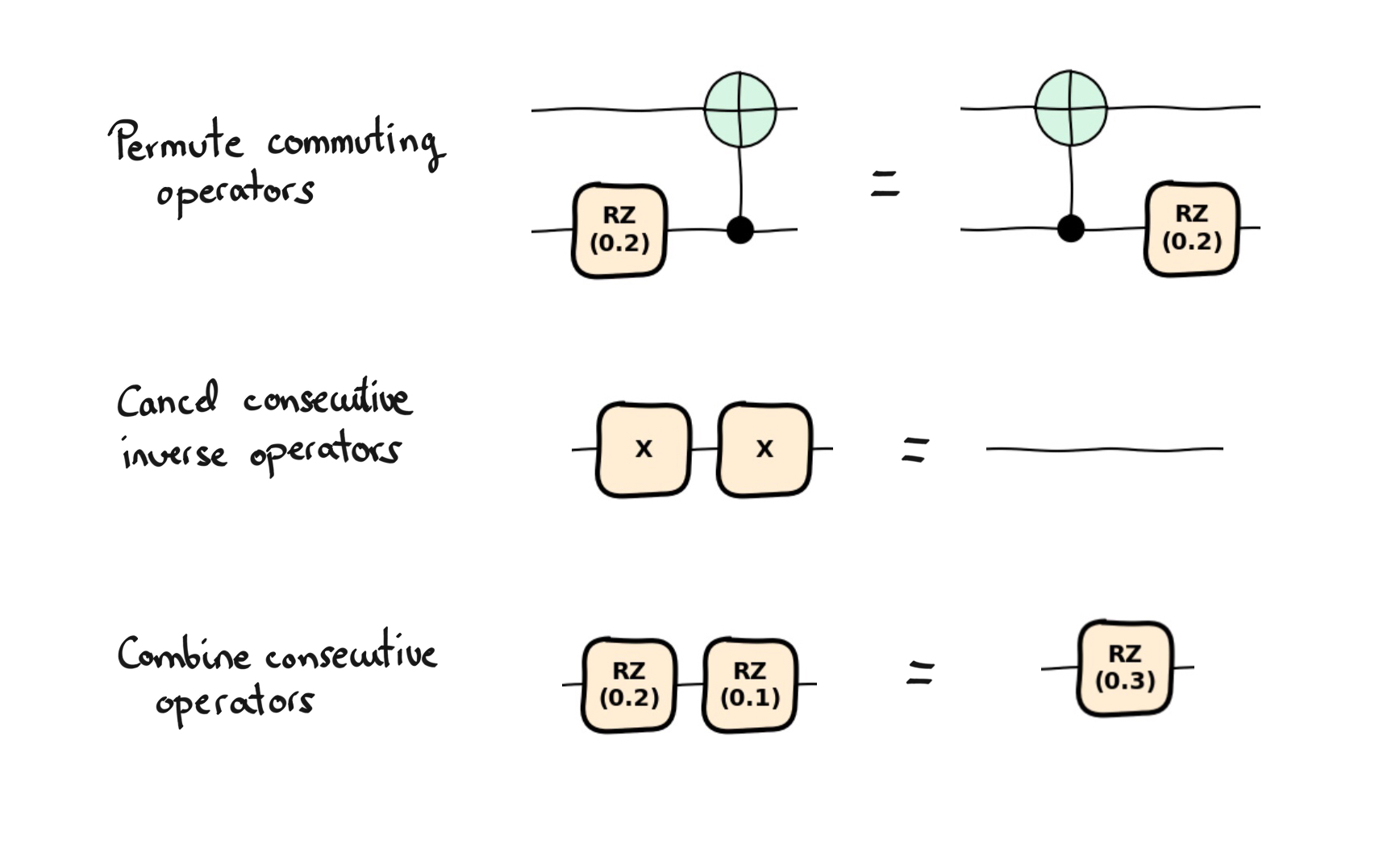
To illustrate their combined effect, let us consider the following circuit.

import pennylane as qml
import matplotlib.pyplot as plt

dev = qml.device("default.qubit", wires=3)


def circuit(angles):
    qml.Hadamard(wires=1)
    qml.Hadamard(wires=2)
    qml.RX(angles[0], 0)
    qml.CNOT(wires=[1, 0])
    qml.CNOT(wires=[2, 1])
    qml.RX(angles[2], wires=0)
    qml.RZ(angles[1], wires=2)
    qml.CNOT(wires=[2, 1])
    qml.RZ(-angles[1], wires=2)
    qml.CNOT(wires=[1, 0])
    qml.Hadamard(wires=1)
    qml.CY(wires=[1, 2])
    qml.CNOT(wires=[1, 0])
    return qml.expval(qml.PauliZ(wires=0))


angles = [0.1, 0.3, 0.5]
qnode = qml.QNode(circuit, dev)
qml.draw_mpl(qnode, decimals=1, style="sketch")(angles)
plt.show()

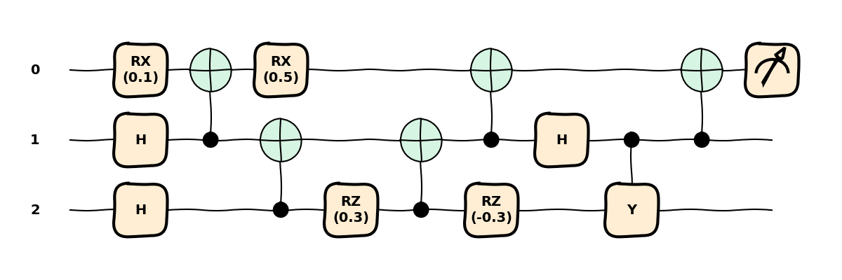
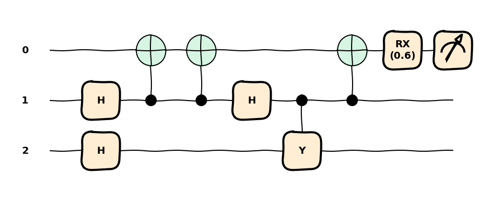
Given an arbitrary quantum circuit, it is usually hard to clearly understand what is really happening. To obtain a better picture, we can shuffle the commuting operations to better distinguish between groups of single-qubit and two-qubit gates. We can easily do so by applying the commute_controlled() transform, which pushes all single-qubit gates towards a direction (defaults to the right).

commuted_circuit = qml.transforms.commute_controlled(direction="right")(circuit)

qnode = qml.QNode(commuted_circuit, dev)
qml.draw_mpl(qnode, decimals=1, style="sketch")(angles)
plt.show()

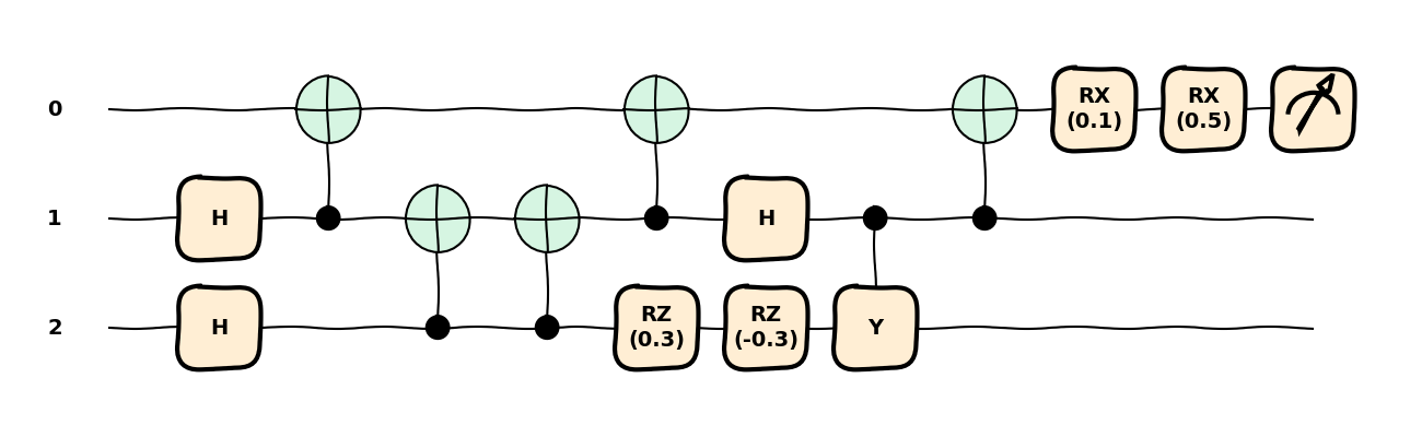
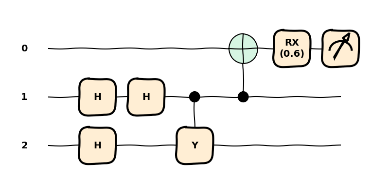
With this rearrangement, we can clearly identify a few operations that can be merged together. For instance, the two consecutive CNOT gates from the third to the second qubits will cancel each other out. We can remove these with the cancel_inverses() transform, which removes consecutive inverse operations.

cancelled_circuit = qml.transforms.cancel_inverses(commuted_circuit)


qnode = qml.QNode(cancelled_circuit, dev)
qml.draw_mpl(qnode, decimals=1, style="sketch")(angles)
plt.show()

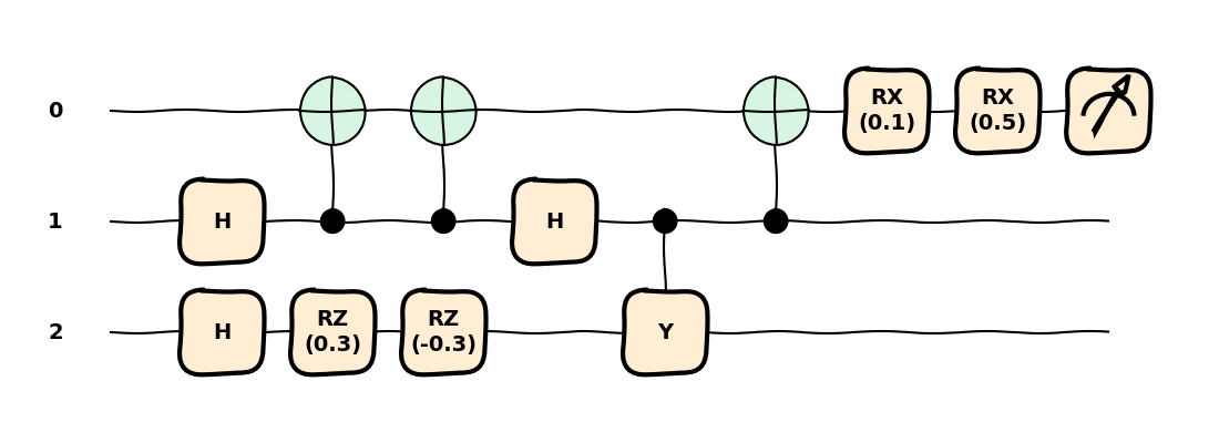
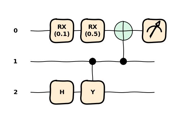
Consecutive rotations along the same axis can also be merged. For example, we can combine the two RX rotations on the first qubit into a single one with the sum of the angles. Additionally, the two RZ rotations on the third qubit will cancel each other. We can combine these rotations with the merge_rotations() transform. We can choose which rotations to merge with include_gates (defaults to None, meaning all). Furthermore, the merged rotations with a resulting angle lower than atol are directly removed.

merged_circuit = qml.transforms.merge_rotations(atol=1e-8, include_gates=None)(cancelled_circuit)


qnode = qml.QNode(merged_circuit, dev)
qml.draw_mpl(qnode, decimals=1, style="sketch")(angles)
plt.show()

Combining these simple circuit transforms, we have reduced the complexity of our original circuit. This will make it faster to execute and less prone to errors. However, there is still room for improvement. Let’s take it a step further in the following section!

As a final remark, we can directly apply the transforms to our quantum function when we define it using their decorator forms (beware the reverse order!).

@qml.qnode(dev)
@qml.transforms.merge_rotations(atol=1e-8, include_gates=None)
@qml.transforms.cancel_inverses
@qml.transforms.commute_controlled(direction="right")
def q_fun(angles):
    qml.Hadamard(wires=1)
    qml.Hadamard(wires=2)
    qml.RX(angles[0], 0)
    qml.CNOT(wires=[1, 0])
    qml.CNOT(wires=[2, 1])
    qml.RX(angles[2], wires=0)
    qml.RZ(angles[1], wires=2)
    qml.CNOT(wires=[2, 1])
    qml.RZ(-angles[1], wires=2)
    qml.CNOT(wires=[1, 0])
    qml.Hadamard(wires=1)
    qml.CY(wires=[1, 2])
    qml.CNOT(wires=[1, 0])
    return qml.expval(qml.PauliZ(wires=0))


qml.draw_mpl(q_fun, decimals=1, style="sketch")(angles)
plt.show()

Circuit compilation

Rearranging and combining operations is an essential part of circuit compilation. Indeed, it is usually performed repeatedly as the compiler does multiple passes over the circuit. During every pass, the compiler applies a series of circuit transforms to obtain better and better circuit representations.

We can apply all the transforms introduced above with the compile() function, which yields the same final circuit.

compiled_circuit = qml.compile()(circuit)

qnode = qml.QNode(compiled_circuit, dev)
qml.draw_mpl(qnode, decimals=1, style="sketch")(angles)
plt.show()

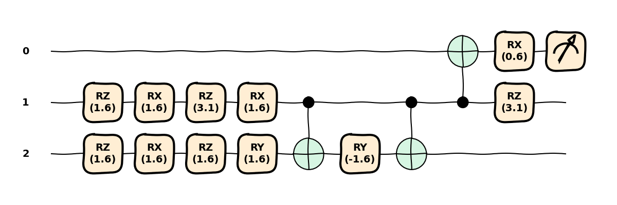
In the resulting circuit, we can identify further operations that can be combined, such as the consecutive CNOT gates applied from the second to the first qubit. To do so, we would simply need to apply the same transforms again in a second pass of the compiler. We can adjust the desired number of passes with num_passes.

Let us see the resulting circuit with two passes.

compiled_circuit = qml.compile(num_passes=2)(circuit)

qnode = qml.QNode(compiled_circuit, dev)
qml.draw_mpl(qnode, decimals=1, style="sketch")(angles)
plt.show()

This can be further simplified with an additional pass of the compiler. In this case, we also define explicitly the transforms to be applied by the compiler with the pipeline argument. This allows us to control the transforms, their parameters, and the order in which they are applied. For example, let’s apply the same transforms in a different order, shift the single-qubit gates towards the opposite direction, and only merge RZ rotations.

compiled_circuit = qml.compile(
    pipeline=[
        qml.transforms.commute_controlled(direction="left"),  # Opposite direction
        qml.transforms.merge_rotations(include_gates=["RZ"]),  # Different threshold
        qml.transforms.cancel_inverses,  # Cancel inverses after rotations
    ],
    num_passes=3,
)(circuit)

qnode = qml.QNode(compiled_circuit, dev)
qml.draw_mpl(qnode, decimals=1, style="sketch")(angles)
plt.show()

Notice how the RX gates on the first qubit have been pushed towards the left and they have not been merged, unlike in the previous cases.

Finally, we can specify a finite basis of gates to describe the circuit by providing a basis_set. For example, suppose we wish to run our circuit on a device that can only implement single-qubit rotations and CNOT operations. In this case, the compiler will need to decompose the gates in terms of our basis, then apply the transforms.

compiled_circuit = qml.compile(basis_set=["CNOT", "RX", "RY", "RZ"], num_passes=2)(circuit)

qnode = qml.QNode(compiled_circuit, dev)
qml.draw_mpl(qnode, decimals=1, style="sketch")(angles)
plt.show()

We can see how the Hadamard and control-Y gates have been decomposed into a series of single-qubit rotations and CNOT gates. We’re ready to run our circuit on the quantum device. Great job!

Conclusion

In this tutorial, we have learned the basic principles of the compilation of quantum circuits. Combining simple circuit transforms that are applied repeatedly during each pass of the compiler, we can significantly reduce the complexity of our quantum circuits.

To continue learning, you can explore other circuit transformations present in the PennyLane transforms module. Furthermore, you can even learn how to create your own in this blogpost.

About the author

Borja Requena

Borja is a PhD student at ICFO - The Institute of Photonic Sciences, where he develops machine learning algorithms to study physics. He is also a summer resident at Xanadu.

demos/tutorial_circuit_compilation

 

Download Python script

 

Download Notebook

 

View on GitHub