Generalization in QML from few training data

Authors: Korbinian Kottmann, Luis Mantilla Calderon, Maurice Weber — Posted: 29 August 2022

In this tutorial, we dive into the generalization capabilities of quantum machine learning models. For the example of a Quantum Convolutional Neural Network (QCNN), we show how its generalization error behaves as a function of the number of training samples. This demo is based on the paper “Generalization in quantum machine learning from few training data”. by Caro et al. 1.

What is generalization in (Q)ML?

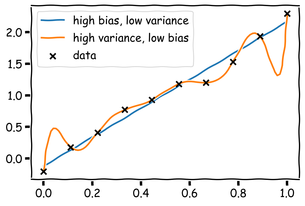
When optimizing a machine learning model, be it classical or quantum, we aim to maximize its performance over the data distribution of interest (e.g., images of cats and dogs). However, in practice, we are limited to a finite amount of data, which is why it is necessary to reason about how our model performs on new, previously unseen data. The difference between the model’s performance on the true data distribution and the performance estimated from our training data is called the generalization error, and it indicates how well the model has learned to generalize to unseen data. Generalization can be seen as a manifestation of the bias-variance trade-off; models that perfectly fit the training data admit a low bias at the cost of a higher variance, and hence typically perform poorly on unseen test data. In the classical machine learning community, this trade-off has been extensively studied and has led to optimization techniques that favour generalization, for example, by regularizing models via their variance 3. Below, we see a canoncial example of this trade-off, with a model having low bias, but high variance and therefore high generalization error. The low variance model, on the other hand, has a higher bias but generalizes better.

Let us now dive deeper into generalization properties of quantum machine learning (QML) models. We start by describing the typical data processing pipeline of a QML model. A classical data input \(x\) is first encoded in a quantum state via a mapping \(x \mapsto \rho(x)\). This encoded state is then processed through a quantum channel \(\rho(x) \mapsto \mathcal{E}_\alpha(\rho(x))\) with learnable parameters \(\alpha\). Finally, a measurement is performed on the resulting state to get the final prediction. Now, the goal is to minimize the expected loss over the data-generating distribution \(P\), indicating how well our model performs on new data. Mathematically, for a loss function \(\ell\), the expected loss, denoted by \(R\), is given by

\[R(\alpha) = \mathbb{E}_{(x,y)\sim P}[\ell(\alpha;\,x,\,y)]\]

where \(x\) are the features, \(y\) are the labels, and \(P\) is their joint distribution. In practice, as the joint distribution \(P\) is generally unknown, this quantity has to be estimated from a finite amount of data. Given a training set \(S = \{(x_i,\,y_i)\}_{i=1}^N\) with \(N\) samples, we estimate the performance of our QML model by calculating the average loss over the training set

\[R_S(\alpha) = \frac{1}{N}\sum_{i=1}^N \ell(\alpha;\,x_i,\,y_i),\]

which is referred to as the training loss and is an unbiased estimate of \(R(\alpha)\). This is only a proxy to the true quantity of interest \(R(\alpha)\), and their difference is called the generalization error

\[\mathrm{gen}(\alpha) = R(\alpha) - \hat{R}_S(\alpha),\]

which is the quantity that we explore in this tutorial. Keeping in mind the bias-variance trade-off, one would expect that more complex models, i.e. models with a larger number of parameters, achieve a lower error on the training data but a higher generalization error. Having more training data, on the other hand, leads to a better approximation of the true expected loss and hence a lower generalization error. This intuition is made precise in Ref. 1, where it is shown that \(\mathrm{gen}(\alpha)\) roughly scales as \(\mathcal{O}(\sqrt{T / N})\), where \(T\) is the number of parametrized gates and \(N\) is the number of training samples.

Generalization bounds for QML models

As hinted at earlier, we expect the generalization error to depend both on the richness of the model class, as well as on the amount of training data available. As a first result, the authors of Ref. 1 found that for a QML model with at most \(T\) parametrized local quantum channels, the generalization error depends on \(T\) and \(N\) according to

\[\mathrm{gen}(\alpha) \sim \mathcal{O}\left(\sqrt{\frac{T\log T}{N}}\right).\]

We see that this scaling is in line with our intuition that the generalization error scales inversely with the number of training samples and increases with the number of parametrized gates. However, as is the case for quantum convolutional neural networks (QCNNs), it is possible to get a more fine-grained bound by including knowledge on the number of gates \(M\) which have been reused (i.e. whose parameters are shared across wires). Naively, one could suspect that the generalization error scales as \(\tilde{\mathcal{O}}(\sqrt{MT/N})\) by directly applying the above result (and where \(\tilde{\mathcal{O}}\) includes logarithmic factors). However, the authors of Ref. 1 found that such models actually adhere to the better scaling

\[\mathrm{gen}(\alpha) \sim \mathcal{O}\left(\sqrt{\frac{T\log MT}{N}}\right).\]

With this, we see that for QCNNs to have a generalization error \(\mathrm{gen}(\alpha)\leq\epsilon\), we need a training set of size \(N \sim T \log MT / \epsilon^2\). For the special case of QCNNs, we can explicitly connect the number of samples needed for good generalization to the system size \(n\) since these models use \(\mathcal{O}(\log(n))\) independently parametrized gates, each of which is used at most \(n\) times 4. Putting the pieces together, we find that a training set of size

\[N \sim \mathcal{O}(\mathrm{poly}(\log n))\]

is sufficient for the generalization error to be bounded by \(\mathrm{gen}(\alpha) \leq \epsilon\). In the next part of this tutorial, we will illustrate this result by implementing a QCNN to classify different digits in the classical digits dataset. Before that, we set up our QCNN.

Quantum convolutional neural networks

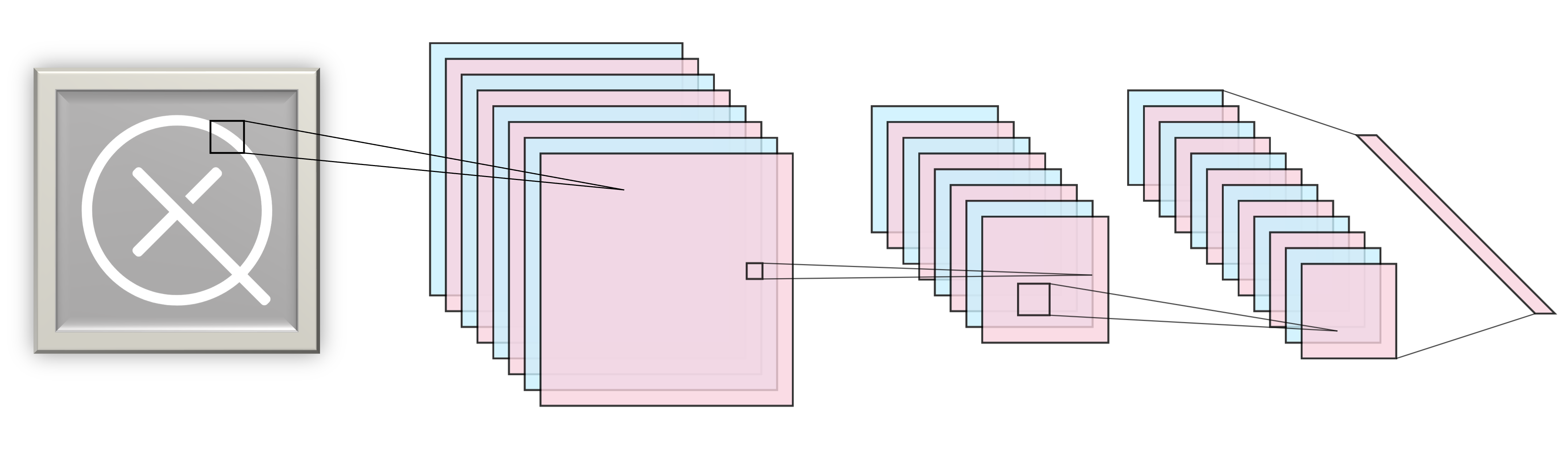
Before we start building a QCNN, let us briefly review the idea of classical CNNs, which have shown tremendous success in tasks like image recognition, recommender systems, and sound classification, to name a few. For a more in-depth explanation of CNNs, we highly recommend chapter 9 in 2. Classical CNNs are a family of neural networks which make use of convolutions and pooling operations to insert an inductive bias, favouring invariances to spatial transformations like translations, rotations, and scaling. A convolutional layer consists of a small kernel (a window) that sweeps over a 2D array representation of an image and extracts local information while sharing parameters across the spatial dimensions. In addition to the convolutional layers, one typically uses pooling layers to reduce the size of the input and to provide a mechanism for summarizing information from a neighbourhood of values in the input. On top of reducing dimensionality, these types of layers have the advantage of making the model more agnostic to certain transformations like scaling and rotations. These two types of layers are applied repeatedly in an alternating manner as shown in the figure below.

A graphical representation of a CNN. Obtained using Ref. 5.

We want to build something similar for a quantum circuit. First, we import the necessary libraries we will need in this demo and set a random seed for reproducibility:

import matplotlib as mpl
import matplotlib.pyplot as plt
import numpy as np
import pandas as pd
from sklearn import datasets
import seaborn as sns
import jax;

jax.config.update('jax_platform_name', 'cpu')
jax.config.update("jax_enable_x64", True)
import jax.numpy as jnp

import optax  # optimization using jax

import pennylane as qml
import pennylane.numpy as pnp

sns.set()

seed = 0
rng = np.random.default_rng(seed=seed)

Out:

/home/runner/work/qml/qml/venv/lib/python3.9/site-packages/seaborn/cm.py:1055: UserWarning: Trying to register the cmap 'rocket' which already exists.
  mpl_cm.register_cmap(_name, _cmap)
/home/runner/work/qml/qml/venv/lib/python3.9/site-packages/seaborn/cm.py:1056: UserWarning: Trying to register the cmap 'rocket_r' which already exists.
  mpl_cm.register_cmap(_name + "_r", _cmap_r)
/home/runner/work/qml/qml/venv/lib/python3.9/site-packages/seaborn/cm.py:1055: UserWarning: Trying to register the cmap 'mako' which already exists.
  mpl_cm.register_cmap(_name, _cmap)
/home/runner/work/qml/qml/venv/lib/python3.9/site-packages/seaborn/cm.py:1056: UserWarning: Trying to register the cmap 'mako_r' which already exists.
  mpl_cm.register_cmap(_name + "_r", _cmap_r)
/home/runner/work/qml/qml/venv/lib/python3.9/site-packages/seaborn/cm.py:1055: UserWarning: Trying to register the cmap 'vlag' which already exists.
  mpl_cm.register_cmap(_name, _cmap)
/home/runner/work/qml/qml/venv/lib/python3.9/site-packages/seaborn/cm.py:1056: UserWarning: Trying to register the cmap 'vlag_r' which already exists.
  mpl_cm.register_cmap(_name + "_r", _cmap_r)
/home/runner/work/qml/qml/venv/lib/python3.9/site-packages/seaborn/cm.py:1055: UserWarning: Trying to register the cmap 'icefire' which already exists.
  mpl_cm.register_cmap(_name, _cmap)
/home/runner/work/qml/qml/venv/lib/python3.9/site-packages/seaborn/cm.py:1056: UserWarning: Trying to register the cmap 'icefire_r' which already exists.
  mpl_cm.register_cmap(_name + "_r", _cmap_r)

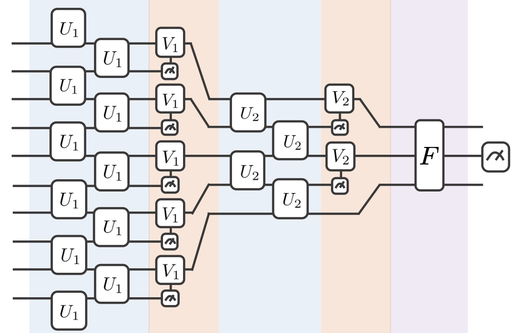
To construct a convolutional and pooling layer in a quantum circuit, we will follow the QCNN construction proposed in 4. The former layer will extract local correlations, while the latter allows reducing the dimensionality of the feature vector. In a quantum circuit, the convolutional layer, consisting of a kernel swept along the entire image, is a two-qubit unitary that correlates neighbouring qubits. As for the pooling layer, we will use a conditioned single-qubit unitary that depends on the measurement of a neighboring qubit. Finally, we use a dense layer that entangles all qubits of the final state using an all-to-all unitary gate as shown in the figure below.

QCNN architecture. Taken from Ref. 4.

Breaking down the layers

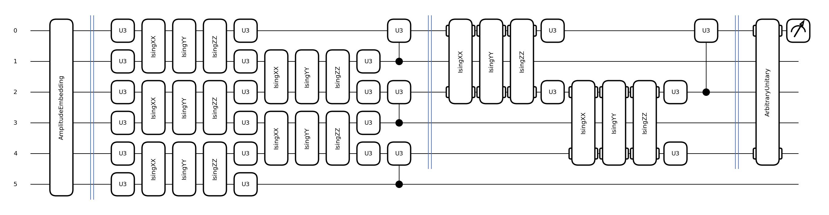
The convolutional layer should have the weights of the two-qubit unitary as an input, which are updated at every training step. In PennyLane, we model this arbitrary two-qubit unitary with a particular sequence of gates: two single-qubit U3 gates (parametrized by three parameters, each), three Ising interactions between both qubits (each interaction is parametrized by one parameter), and two additional U3 gates on each of the two qubits.

def convolutional_layer(weights, wires, skip_first_layer=True):
    """Adds a convolutional layer to a circuit.
    Args:
        weights (np.array): 1D array with 15 weights of the parametrized gates.
        wires (list[int]): Wires where the convolutional layer acts on.
        skip_first_layer (bool): Skips the first two U3 gates of a layer.
    """
    n_wires = len(wires)
    assert n_wires >= 3, "this circuit is too small!"

    for p in [0, 1]:
        for indx, w in enumerate(wires):
            if indx % 2 == p and indx < n_wires - 1:
                if indx % 2 == 0 and not skip_first_layer:
                    qml.U3(*weights[:3], wires=[w])
                    qml.U3(*weights[3:6], wires=[wires[indx + 1]])
                qml.IsingXX(weights[6], wires=[w, wires[indx + 1]])
                qml.IsingYY(weights[7], wires=[w, wires[indx + 1]])
                qml.IsingZZ(weights[8], wires=[w, wires[indx + 1]])
                qml.U3(*weights[9:12], wires=[w])
                qml.U3(*weights[12:], wires=[wires[indx + 1]])

The pooling layer’s inputs are the weights of the single-qubit conditional unitaries, which in this case are U3 gates. Then, we apply these conditional measurements to half of the unmeasured wires, reducing our system size by a factor of 2.

def pooling_layer(weights, wires):
    """Adds a pooling layer to a circuit.
    Args:
        weights (np.array): Array with the weights of the conditional U3 gate.
        wires (list[int]): List of wires to apply the pooling layer on.
    """
    n_wires = len(wires)
    assert len(wires) >= 2, "this circuit is too small!"

    for indx, w in enumerate(wires):
        if indx % 2 == 1 and indx < n_wires:
            m_outcome = qml.measure(w)
            qml.cond(m_outcome, qml.U3)(*weights, wires=wires[indx - 1])

We can construct a QCNN by combining both layers and using an arbitrary unitary to model a dense layer. It will take a set of features — the image — as input, encode these features using an embedding map, apply rounds of convolutional and pooling layers, and eventually output the desired measurement statistics of the circuit.

def conv_and_pooling(kernel_weights, n_wires, skip_first_layer=True):
    """Apply both the convolutional and pooling layer."""
    convolutional_layer(kernel_weights[:15], n_wires, skip_first_layer=skip_first_layer)
    pooling_layer(kernel_weights[15:], n_wires)


def dense_layer(weights, wires):
    """Apply an arbitrary unitary gate to a specified set of wires."""
    qml.ArbitraryUnitary(weights, wires)


num_wires = 6
device = qml.device("default.qubit", wires=num_wires)


@qml.qnode(device, interface="jax")
def conv_net(weights, last_layer_weights, features):
    """Define the QCNN circuit
    Args:
        weights (np.array): Parameters of the convolution and pool layers.
        last_layer_weights (np.array): Parameters of the last dense layer.
        features (np.array): Input data to be embedded using AmplitudEmbedding."""

    layers = weights.shape[1]
    wires = list(range(num_wires))

    # inputs the state input_state
    qml.AmplitudeEmbedding(features=features, wires=wires, pad_with=0.5)
    qml.Barrier(wires=wires, only_visual=True)

    # adds convolutional and pooling layers
    for j in range(layers):
        conv_and_pooling(weights[:, j], wires, skip_first_layer=(not j == 0))
        wires = wires[::2]
        qml.Barrier(wires=wires, only_visual=True)

    assert last_layer_weights.size == 4 ** (len(wires)) - 1, (
        "The size of the last layer weights vector is incorrect!"
        f" \n Expected {4 ** (len(wires)) - 1}, Given {last_layer_weights.size}"
    )
    dense_layer(last_layer_weights, wires)
    return qml.probs(wires=(0))


fig, ax = qml.draw_mpl(conv_net)(
    np.random.rand(18, 2), np.random.rand(4 ** 2 - 1), np.random.rand(2 ** num_wires)
)
plt.show()

In the problem we will address, we need to encode 64 features in our quantum state. Thus, we require six qubits (\(2^6 = 64\)) to encode each feature value in the amplitude of each computational basis state.

Training the QCNN on the digits dataset

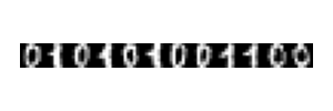
In this demo, we are going to classify the digits 0 and 1 from the classical digits dataset. Each hand-written digit image is represented as an \(8 \times 8\) array of pixels as shown below:

digits = datasets.load_digits()
images, labels = digits.data, digits.target

images = images[np.where((labels == 0) | (labels == 1))]
labels = labels[np.where((labels == 0) | (labels == 1))]

fig, axes = plt.subplots(nrows=1, ncols=12, figsize=(3, 1))

for i, ax in enumerate(axes.flatten()):
    ax.imshow(images[i].reshape((8, 8)), cmap="gray")
    ax.axis("off")

plt.tight_layout()
plt.subplots_adjust(wspace=0, hspace=0)
plt.show()

For convenience, we create a load_digits_data function that will make random training and testing sets from the digits dataset from sklearn.dataset:

def load_digits_data(num_train, num_test, rng):
    """Return training and testing data of digits dataset."""
    digits = datasets.load_digits()
    features, labels = digits.data, digits.target

    # only use first two classes
    features = features[np.where((labels == 0) | (labels == 1))]
    labels = labels[np.where((labels == 0) | (labels == 1))]

    # normalize data
    features = features / np.linalg.norm(features, axis=1).reshape((-1, 1))

    # subsample train and test split
    train_indices = rng.choice(len(labels), num_train, replace=False)
    test_indices = rng.choice(
        np.setdiff1d(range(len(labels)), train_indices), num_test, replace=False
    )

    x_train, y_train = features[train_indices], labels[train_indices]
    x_test, y_test = features[test_indices], labels[test_indices]

    return (
        jnp.asarray(x_train),
        jnp.asarray(y_train),
        jnp.asarray(x_test),
        jnp.asarray(y_test),
    )

To optimize the weights of our variational model, we define the cost and accuracy functions to train and quantify the performance on the classification task of the previously described QCNN:

@jax.jit
def compute_out(weights, weights_last, features, labels):
    """Computes the output of the corresponding label in the qcnn"""
    cost = lambda weights, weights_last, feature, label: conv_net(weights, weights_last, feature)[
        label
    ]
    return jax.vmap(cost, in_axes=(None, None, 0, 0), out_axes=0)(
        weights, weights_last, features, labels
    )


def compute_accuracy(weights, weights_last, features, labels):
    """Computes the accuracy over the provided features and labels"""
    out = compute_out(weights, weights_last, features, labels)
    return jnp.sum(out > 0.5) / len(out)


def compute_cost(weights, weights_last, features, labels):
    """Computes the cost over the provided features and labels"""
    out = compute_out(weights, weights_last, features, labels)
    return 1.0 - jnp.sum(out) / len(labels)


def init_weights():
    """Initializes random weights for the QCNN model."""
    weights = pnp.random.normal(loc=0, scale=1, size=(18, 2), requires_grad=True)
    weights_last = pnp.random.normal(loc=0, scale=1, size=4 ** 2 - 1, requires_grad=True)
    return jnp.array(weights), jnp.array(weights_last)


value_and_grad = jax.jit(jax.value_and_grad(compute_cost, argnums=[0, 1]))

We are going to perform the classification for training sets with different values of \(N\). Therefore, we define the classification procedure once and then perform it for different datasets. Finally, we update the weights using the pennylane.AdamOptimizer and use these updated weights to calculate the cost and accuracy on the testing and training set:

def train_qcnn(n_train, n_test, n_epochs):
    """
    Args:
        n_train  (int): number of training examples
        n_test   (int): number of test examples
        n_epochs (int): number of training epochs
        desc  (string): displayed string during optimization

    Returns:
        dict: n_train,
        steps,
        train_cost_epochs,
        train_acc_epochs,
        test_cost_epochs,
        test_acc_epochs

    """
    # load data
    x_train, y_train, x_test, y_test = load_digits_data(n_train, n_test, rng)

    # init weights and optimizer
    weights, weights_last = init_weights()

    # learning rate decay
    cosine_decay_scheduler = optax.cosine_decay_schedule(0.1, decay_steps=n_epochs, alpha=0.95)
    optimizer = optax.adam(learning_rate=cosine_decay_scheduler)
    opt_state = optimizer.init((weights, weights_last))

    # data containers
    train_cost_epochs, test_cost_epochs, train_acc_epochs, test_acc_epochs = [], [], [], []

    for step in range(n_epochs):
        # Training step with (adam) optimizer
        train_cost, grad_circuit = value_and_grad(weights, weights_last, x_train, y_train)
        updates, opt_state = optimizer.update(grad_circuit, opt_state)
        weights, weights_last = optax.apply_updates((weights, weights_last), updates)

        train_cost_epochs.append(train_cost)

        # compute accuracy on training data
        train_acc = compute_accuracy(weights, weights_last, x_train, y_train)
        train_acc_epochs.append(train_acc)

        # compute accuracy and cost on testing data
        test_out = compute_out(weights, weights_last, x_test, y_test)
        test_acc = jnp.sum(test_out > 0.5) / len(test_out)
        test_acc_epochs.append(test_acc)
        test_cost = 1.0 - jnp.sum(test_out) / len(test_out)
        test_cost_epochs.append(test_cost)

    return dict(
        n_train=[n_train] * n_epochs,
        step=np.arange(1, n_epochs + 1, dtype=int),
        train_cost=train_cost_epochs,
        train_acc=train_acc_epochs,
        test_cost=test_cost_epochs,
        test_acc=test_acc_epochs,
    )

Note

There are some small intricacies for speeding up this code that are worth mentioning. We are using jax for our training because it allows for just-in-time (jit) compilation. A function decorated with @jax.jit will be compiled upon its first execution and cached for future executions. This means the first execution will take longer, but all subsequent executions are substantially faster. Further, we use jax.vmap to vectorize the execution of the QCNN over all input states, as opposed to looping through the training and test set at every execution.

Training for different training set sizes yields different accuracies, as seen below. As we increase the training data size, the overall test accuracy, a proxy for the models’ generalization capabilities, increases:

n_test = 100
n_epochs = 100
n_reps = 100


def run_iterations(n_train):
    results_df = pd.DataFrame(
        columns=["train_acc", "train_cost", "test_acc", "test_cost", "step", "n_train"]
    )

    for _ in range(n_reps):
        results = train_qcnn(n_train=n_train, n_test=n_test, n_epochs=n_epochs)
        results_df = pd.concat(
            [results_df, pd.DataFrame.from_dict(results)], axis=0, ignore_index=True
        )

    return results_df


# run training for multiple sizes
train_sizes = [2, 5, 10, 20, 40, 80]
results_df = run_iterations(n_train=2)
for n_train in train_sizes[1:]:
    results_df = pd.concat([results_df, run_iterations(n_train=n_train)])

Finally, we plot the loss and accuracy for both the training and testing set for all training epochs, and compare the test and train accuracy of the model:

# aggregate dataframe
df_agg = results_df.groupby(["n_train", "step"]).agg(["mean", "std"])
df_agg = df_agg.reset_index()

sns.set_style('whitegrid')
colors = sns.color_palette()
fig, axes = plt.subplots(ncols=3, figsize=(16.5, 5))

generalization_errors = []

# plot losses and accuracies
for i, n_train in enumerate(train_sizes):
    df = df_agg[df_agg.n_train == n_train]

    dfs = [df.train_cost["mean"], df.test_cost["mean"], df.train_acc["mean"], df.test_acc["mean"]]
    lines = ["o-", "x--", "o-", "x--"]
    labels = [fr"$N={n_train}$", None, fr"$N={n_train}$", None]
    axs = [0,0,2,2]

    for k in range(4):
        ax = axes[axs[k]]
        ax.plot(df.step, dfs[k], lines[k], label=labels[k], markevery=10, color=colors[i], alpha=0.8)


    # plot final loss difference
    dif = df[df.step == 100].test_cost["mean"] - df[df.step == 100].train_cost["mean"]
    generalization_errors.append(dif)

# format loss plot
ax = axes[0]
ax.set_title('Train and Test Losses', fontsize=14)
ax.set_xlabel('Epoch')
ax.set_ylabel('Loss')

# format generalization error plot
ax = axes[1]
ax.plot(train_sizes, generalization_errors, "o-", label=r"$gen(\alpha)$")
ax.set_xscale('log')
ax.set_xticks(train_sizes)
ax.set_xticklabels(train_sizes)
ax.set_title(r'Generalization Error $gen(\alpha) = R(\alpha) - \hat{R}_N(\alpha)$', fontsize=14)
ax.set_xlabel('Training Set Size')

# format loss plot
ax = axes[2]
ax.set_title('Train and Test Accuracies', fontsize=14)
ax.set_xlabel('Epoch')
ax.set_ylabel('Accuracy')
ax.set_ylim(0.5, 1.05)

legend_elements = [
    mpl.lines.Line2D([0], [0], label=f'N={n}', color=colors[i]) for i, n in enumerate(train_sizes)
    ] + [
    mpl.lines.Line2D([0], [0], marker='o', ls='-', label='Train', color='Black'),
    mpl.lines.Line2D([0], [0], marker='x', ls='--', label='Test', color='Black')
    ]

axes[0].legend(handles=legend_elements, ncol=3)
axes[2].legend(handles=legend_elements, ncol=3)

axes[1].set_yscale('log', base=2)
plt.show()

---

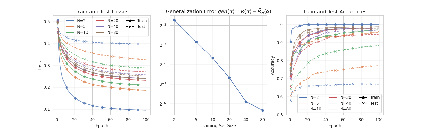
The key takeaway of this work is that some quantum learning models can achieve high-fidelity predictions using a few training data points. We implemented a model known as the quantum convolutional neural network (QCNN) using PennyLane for a binary classification task. Using six qubits, we have trained the QCNN to distinguish between handwritten digits of \(0\)’s and \(1\)’s. With \(80\) samples, we have achieved a model with accuracy greater than \(97\%\) in \(100\) training epochs. Furthermore, we have compared the test and train accuracy of this model for a different number of training samples and found the scaling of the generalization error agrees with the theoretical bounds obtained in 1.

References

1(1,2,3,4,5)

Matthias C. Caro, Hsin-Yuan Huang, M. Cerezo, Kunal Sharma, Andrew Sornborger, Lukasz Cincio, Patrick J. Coles. “Generalization in quantum machine learning from few training data” arxiv:2111.05292, 2021.

2

Ian Goodfellow, Yoshua Bengio and Aaron Courville. “Deep Learning”2, 2016.

3

Hongseok Namkoong and John C. Duchi. “Variance-based regularization with convex objectives.” Advances in Neural Information Processing Systems, 2017.

4(1,2,3)

Iris Cong, Soonwon Choi, Mikhail D. Lukin. “Quantum Convolutional Neural Networks” arxiv:1810.03787, 2018.

5

Alexander LeNail. “NN-SVG: Publication-Ready Neural Network Architecture Schematics” Journal of Open Source Software, 2019.

About the authors

Korbinian Kottmann

Korbinian is a Quantum Scientist at Xanadu, interested in quantum simulation and quantum software.

Luis Mantilla Calderon

Luis is a summer resident at Xanadu. He works in quantum error correction and is interested in QML, quantum compilation, and BCI technology.

Maurice Weber

Maurice is a summer resident at Xanadu and a PhD student at ETH Zürich. He is interested in the intersection of Machine Learning and Quantum Computing.

demos/tutorial_learning_few_data

 

Download Python script

 

Download Notebook

 

View on GitHub