Function Fitting using Quantum Signal Processing

Author: Jay Soni — Posted: 24 May 2022. Last updated: 17 April 2023.

Introduction

This demo is inspired by the paper ‘A Grand Unification of Quantum Algorithms’. This paper is centered around the Quantum Singular Value Transform (QSVT) protocol and how it provides a single framework to generalize some of the most famous quantum algorithms like Shor’s factoring algorithm, Grover search, and more.

The QSVT is a method to apply polynomial transformations to the singular values of any matrix. This is powerful because from polynomial transformations we can generate arbitrary function transformations using Taylor approximations. The QSVT protocol is an extension of the more constrained Quantum Signal Processing (QSP) protocol which presents a method for polynomial transformation of matrix entries in a single-qubit unitary operator. The QSVT protocol is sophisticated, but the idea at its core is quite simple. By studying QSP, we get a relatively simpler path to explore this idea at the foundation of QSVT.

In this demo, we explore the QSP protocol and how it can be used for curve fitting. We show how you can fit polynomials, as illustrated in the animation below.

This is a powerful tool that will ultimately allow us to approximate any function on the interval \([-1, 1]\) that satisfies certain constraints. Before we can dive into function fitting, let’s develop some intuition. Consider the following single-qubit operator parameterized by \(a \in [-1, 1]\):

\[\begin{split}\hat{W}(a) = \begin{bmatrix} a & i\sqrt{1 - a^{2}} \\ i\sqrt{1 - a^{2}} & a \end{bmatrix}.\end{split}\]

\(\hat{W}(a)\) is called the signal rotation operator (SRO). Using this operator, we can construct another operator which we call signal processing operator (SPO),

\[\hat{U}_{sp} = \hat{R}_{z}(\phi_{0}) \prod_{k=1}^{d} \hat{W}(a) \hat{R}_{z}(\phi_{k}).\]

The SPO is parameterized by a vector \(\vec{\phi} \in \mathbb{R}^{d+1}\), where \(d\) is a free parameter which represents the number of repeated applications of \(\hat{W}(a)\).

The SPO \(\hat{U}_{sp}\) alternates between applying the SRO \(\hat{W}(a)\) and parameterized rotations around the z-axis. Let’s see what happens when we try to compute the expectation value \(\langle 0|\hat{U}_{sp}|0\rangle\) for the particular case where \(d = 2\) and \(\vec{\phi} = (0, 0, 0)\) :

\[\begin{split}\begin{align*} \langle 0 |\hat{U}_{sp}|0\rangle &= \langle 0 | \ \hat{R}_{z}(0) \prod_{k=1}^{2} \hat{W}(a) \hat{R}_{z}(0) \ |0\rangle \\ \langle 0 |\hat{U}_{sp}|0\rangle &= \langle 0 | \hat{W}(a)^{2} |0\rangle \\ \end{align*}\end{split}\]

\[\begin{split}\langle 0 |\hat{U}_{sp}|0\rangle = \langle 0 | \begin{bmatrix} a & i\sqrt{1 - a^{2}} \\ i\sqrt{1 - a^{2}} & a \end{bmatrix} \ \circ \ \begin{bmatrix} a & i\sqrt{1 - a^{2}} \\ i\sqrt{1 - a^{2}} & a \end{bmatrix} |0\rangle\end{split}\]

\[\begin{split}\langle 0|\hat{U}_{sp}|0\rangle = \langle 0| \begin{bmatrix} 2a^{2} - 1 & 2ai\sqrt{1 - a^{2}} \\ 2ai\sqrt{1 - a^{2}} & 2a^{2} - 1 \end{bmatrix} |0\rangle\end{split}\]

\[\langle 0|\hat{U}_{sp}|0\rangle = 2a^{2} - 1\]

Notice that this quantity is a polynomial in \(a\). Equivalently, suppose we wanted to create a map \(S: a \to 2a^2 - 1\). This expectation value would give us the means to perform such a mapping. This may seem oddly specific at first, but it turns out that this process can be generalized for generating a mapping \(S: a \to \text{poly}(a)\). The following theorem shows us how:

Theorem: Quantum Signal Processing

Given a vector \(\vec{\phi} \in \mathbb{R}^{d+1}\), there exist complex polynomials \(P(a)\) and \(Q(a)\) such that the SPO, \(\hat{U}_{sp}\), can be expressed in matrix form as:

\[\hat{U}_{sp} = \hat{R}_{z}(\phi_{0}) \prod_{k=1}^{d} \hat{W}(a) \hat{R}_{z}(\phi_{k}),\]

\[\begin{split}\hat{U}_{sp} = \begin{bmatrix} P(a) & iQ(a)\sqrt{1 - a^{2}} \\ iQ^{*}(a)\sqrt{1 - a^{2}} & P^{*}(a) \end{bmatrix},\end{split}\]

where \(a \in [-1, 1]\) and the polynomials \(P(a)\), \(Q(a)\) satisfy the following constraints:

• \(deg(P) \leq d \ \) and \(deg(Q) \leq d - 1\),

• \(P\) has parity \(d\) mod 2 and \(Q\) has parity, \(d - 1\) mod 2

• \(|P|^{2} + (1 - a^{2})|Q|^{2} = 1\).

The third condition is actually quite restrictive because if we substitute \(a = \pm 1\), we get the result \(|P^{2}(\pm 1)| = 1\). Thus it restricts the polynomial to be pinned to \(\pm 1\) at the end points of the domain, \(a = \pm 1\). This condition can be relaxed to \(|P^{2}(a)| \leq 1\) by expressing the signal processing operator in the Hadamard basis, i.e., \(\langle + |\hat{U}_{sp}(\vec{\phi};a)|+\rangle\)). This is equivalent to redefining \(P(a)\) such that:

\[P^{'}(a) = \text{Re}(P(a)) + i\text{Re}(Q(a))\sqrt{1 - a^{2}}\]

This is the convention we follow in this demo.

Let’s Plot some Polynomials

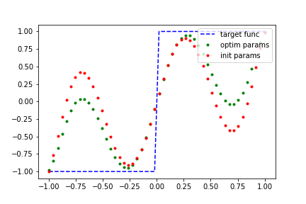
Now we put this theorem to the test! In this section we construct the SRO \(\hat{W}(a)\), and then use PennyLane to define the SPO. To test the theorem we will randomly generate parameters \(\vec{\phi}\) and plot the expectation value \(\langle + |\hat{U}_{sp}(\vec{\phi};a)|+\rangle\) for \(a \in [-1, 1]\).

Next, we introduce a function called rotation_mat(a), which will construct the SRO matrix. We can also make a helper function (generate_many_sro(a_vals)) which, given an array of possible values for ‘\(a\)’, will generate an array of \(\hat{W}(a)\) associated with each element. We use Pytorch to construct this array as it will later be used as input when training our function fitting model.

import torch


def rotation_mat(a):
    """Given a fixed value 'a', compute the signal rotation matrix W(a).
    (requires -1 <= 'a' <= 1)
    """
    diag = a
    off_diag = (1 - a**2) ** (1 / 2) * 1j
    W = [[diag, off_diag], [off_diag, diag]]

    return W


def generate_many_sro(a_vals):
    """Given a tensor of possible 'a' vals, return a tensor of W(a)"""
    w_array = []
    for a in a_vals:
        w = rotation_mat(a)
        w_array.append(w)

    return torch.tensor(w_array, dtype=torch.complex64, requires_grad=False)

Now having access to the matrix elements of the SRO, we can leverage PennyLane to define a quantum function that will compute the SPO. Recall we are measuring in the Hadamard basis to relax the third condition of the theorem. We accomplish this by sandwiching the SPO between two Hadamard gates to account for this change of basis.

import pennylane as qml


def QSP_circ(phi, W):
    """This circuit applies the SPO. The components in the matrix
    representation of the final unitary are polynomials!
    """
    qml.Hadamard(wires=0)  # set initial state |+>
    for angle in phi[:-1]:
        qml.RZ(angle, wires=0)
        qml.QubitUnitary(W, wires=0)

    qml.RZ(phi[-1], wires=0)  # final rotation
    qml.Hadamard(wires=0)  # change of basis |+> , |->
    return

Finally, we randomly generate the vector \(\vec{\phi}\) and plot the expectation value \(\langle +|\hat{U}_{sp}|+\rangle\) as a function of \(a\). In this case we choose \(d = 5\). We expect to observe the following:

• Since \(d\) is odd, we expect all of the polynomials we plot to have odd symmetry

• Since \(d = 5\), we expect none of the polynomials will have terms ~ \(O(a^6)\) or higher

• All of the polynomials are bounded by \(\pm1\)

import math
import matplotlib.pyplot as plt

d = 5
a_vals = torch.linspace(-1, 1, 50)
w_mats = generate_many_sro(a_vals)

gen = torch.Generator()
gen.manual_seed(444422)  # set random seed for reproducibility

for i in range(5):
    phi = torch.rand(d + 1, generator=gen) * 2 * torch.tensor([math.pi], requires_grad=False)
    matrix_func = qml.matrix(QSP_circ)
    y_vals = [matrix_func(phi, w)[0, 0].real for w in w_mats]

    plt.plot(a_vals, y_vals, label=f"poly #{i}")

plt.vlines(0.0, -1.0, 1.0, color="black")
plt.hlines(0.0, -1.0, 1.0, color="black")
plt.legend(loc=1)
plt.show()

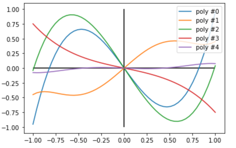
Exactly as predicted, all of these conditions are met!

• All curves have odd symmetry

• Qualitatively, the plots look similar to polynomials of low degree

• Each plot does not exceed \(\pm1\) !

Function Fitting with Quantum Signal Processing

Another observation we can make about this theorem is the fact that it holds true in both directions: If we have two polynomials \(P(a)\) and \(Q(a)\) that satisfy the conditions of the theorem, then there exists a \(\vec{\phi}\) for which we can construct a signal processing operator which maps \(a \to P(a)\).

In this section we try to answer the question:

Can we learn the parameter values of \(\vec{\phi}\) to transform our signal processing operator polynomial to fit a given function?

In order to answer this question, we leverage the power of machine learning. In this demo we assume you are familiar with some concepts from quantum machine learning, for a refresher checkout this blog post on QML. We begin by building a machine learning model using Pytorch. The __init__() method handles the random initialization of our parameter vector \(\vec{\phi}\). The forward() method takes an array of signal rotation matrices \(\hat{W}(a)\) for varying \(a\), and produces the predicted \(y\) values.

Next we leverage the PennyLane function qml.matrix(), which accepts our quantum function (it can also accept quantum tapes and QNodes) and returns its unitary matrix representation. We are interested in the real value of the top left entry, this corresponds to \(P(a)\).

torch_pi = torch.Tensor([math.pi])


class QSP_Func_Fit(torch.nn.Module):
    def __init__(self, degree, num_vals, random_seed=None):
        """Given the degree and number of samples, this method randomly
        initializes the parameter vector (randomness can be set by random_seed)
        """
        super().__init__()
        if random_seed is None:
            self.phi = torch_pi * torch.rand(degree + 1, requires_grad=True)

        else:
            gen = torch.Generator()
            gen.manual_seed(random_seed)
            self.phi = torch_pi * torch.rand(degree + 1, requires_grad=True, generator=gen)

        self.phi = torch.nn.Parameter(self.phi)
        self.num_phi = degree + 1
        self.num_vals = num_vals

    def forward(self, omega_mats):
        """PennyLane forward implementation"""
        y_pred = []
        generate_qsp_mat = qml.matrix(QSP_circ)

        for w in omega_mats:
            u_qsp = generate_qsp_mat(self.phi, w)
            P_a = u_qsp[0, 0]  # Taking the (0,0) entry of the matrix corresponds to <0|U|0>
            y_pred.append(P_a.real)

        return torch.stack(y_pred, 0)

Next we create a Model_Runner class to handle running the optimization, storing the results, and providing plotting functionality:

class Model_Runner:
    def __init__(self, model, degree, num_samples, x_vals, process_x_vals, y_true):
        """Given a model and a series of model specific arguments, store everything in
        internal attributes.
        """
        self.model = model
        self.degree = degree
        self.num_samples = num_samples

        self.x_vals = x_vals
        self.inp = process_x_vals(x_vals)
        self.y_true = y_true

    def execute(
        self, random_seed=13_02_1967, max_shots=25000, verbose=True
    ):  # easter egg: oddly specific seed?
        """Run the optimization protocol on the model using Mean Square Error as a loss
        function and using stochastic gradient descent as the optimizer.
        """
        model = self.model(degree=self.degree, num_vals=self.num_samples, random_seed=random_seed)

        criterion = torch.nn.MSELoss(reduction="sum")
        optimizer = torch.optim.SGD(model.parameters(), lr=1e-5)

        t = 0
        loss_val = 1.0

        while (t <= max_shots) and (loss_val > 0.5):

            self.y_pred = model(self.inp)

            if t == 1:
                self.init_y_pred = self.y_pred

            # Compute and print loss
            loss = criterion(self.y_pred, self.y_true)
            loss_val = loss.item()

            if (t % 1000 == 0) and verbose:
                print(f"---- iter: {t}, loss: {round(loss_val, 4)} -----")

            # Perform a backward pass and update weights.
            optimizer.zero_grad()
            loss.backward()
            optimizer.step()

            t += 1

        self.model_params = model.phi

    def plot_result(self, show=True):
        """Plot the results"""
        plt.plot(self.x_vals, self.y_true.tolist(), "--b", label="target func")
        plt.plot(self.x_vals, self.y_pred.tolist(), ".g", label="optim params")
        plt.plot(self.x_vals, self.init_y_pred.tolist(), ".r", label="init params")
        plt.legend(loc=1)

        if show:
            plt.show()

Now that we have a model, lets first attempt to fit a polynomial. We expect this to perform well when the target polynomial also obeys the symmetry and degree constraints that our quantum signal processing polynomial does. To do this, we defined a function custom_poly(x) which implements the target polynomial. In this case, we (arbitrarily) choose the target polynomial:

\[y = 4x^{5} - 5x^{3} + x\]

Lets see how well we can fit this polynomial!

Note

Depending on the initial parameters, training can take anywhere from 10 - 30 mins

import numpy as np

d = 9  # dim(phi) = d + 1,
num_samples = 50


def custom_poly(x):
    """A custom polynomial of degree <= d and parity d % 2"""
    return torch.tensor(4 * x**5 - 5 * x**3 + x, requires_grad=False, dtype=torch.float)


a_vals = np.linspace(-1, 1, num_samples)
y_true = custom_poly(a_vals)

qsp_model_runner = Model_Runner(QSP_Func_Fit, d, num_samples, a_vals, generate_many_sro, y_true)

qsp_model_runner.execute()
qsp_model_runner.plot_result()

Out:

---- iter: 0, loss: 13.5938 -----
---- iter: 1000, loss: 11.8809 -----
---- iter: 2000, loss: 10.229 -----
---- iter: 3000, loss: 8.6693 -----
---- iter: 4000, loss: 7.2557 -----
---- iter: 5000, loss: 6.0084 -----
---- iter: 6000, loss: 4.9197 -----
---- iter: 7000, loss: 3.9801 -----
---- iter: 8000, loss: 3.1857 -----
---- iter: 9000, loss: 2.5312 -----
---- iter: 10000, loss: 2.0045 -----
---- iter: 11000, loss: 1.5873 -----
---- iter: 12000, loss: 1.2594 -----
---- iter: 13000, loss: 1.0021 -----
---- iter: 14000, loss: 0.7997 -----
---- iter: 15000, loss: 0.6397 -----
---- iter: 16000, loss: 0.5127 -----

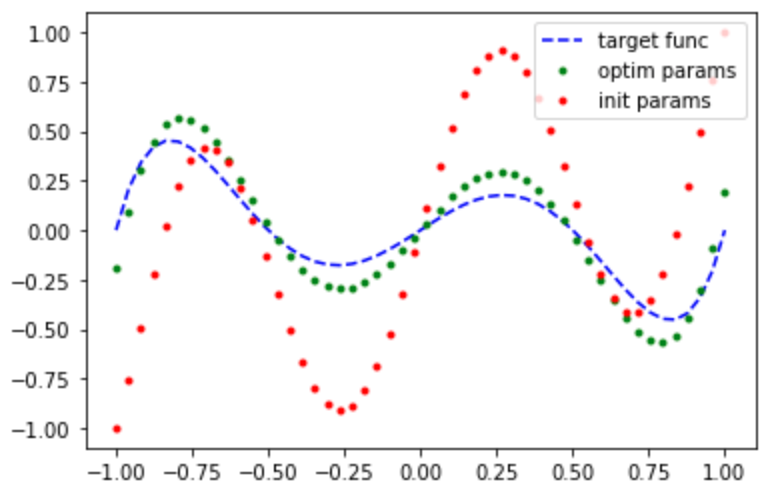
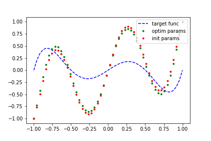
We were able to fit that polynomial quite well! Lets try something more challenging: fitting a non-polynomial function. One thing to keep in mind is the symmetry and bounds constraints on our polynomials. If our target function does not satisfy them as well, then we cannot hope to generate a good polynomial fit, regardless of how long we train for.

A good non-polynomial candidate to fit to, that obeys our constraints, is the step function. Let’s try it!

d = 9  # dim(phi) = d + 1,
num_samples = 50


def step_func(x):
    """A step function (odd parity) which maps all values <= 0 to -1
    and all values > 0 to +1.
    """
    res = [-1.0 if x_i <= 0 else 1.0 for x_i in x]
    return torch.tensor(res, requires_grad=False, dtype=torch.float)


a_vals = np.linspace(-1, 1, num_samples)
y_true = step_func(a_vals)

qsp_model_runner = Model_Runner(QSP_Func_Fit, d, num_samples, a_vals, generate_many_sro, y_true)

qsp_model_runner.execute()
qsp_model_runner.plot_result()

Out:

---- iter: 0, loss: 33.8345 -----
---- iter: 1000, loss: 19.0937 -----
---- iter: 2000, loss: 11.6557 -----
---- iter: 3000, loss: 8.2853 -----
---- iter: 4000, loss: 6.6824 -----
---- iter: 5000, loss: 5.8523 -----
---- iter: 6000, loss: 5.3855 -----
---- iter: 7000, loss: 5.1036 -----
---- iter: 8000, loss: 4.9227 -----
---- iter: 9000, loss: 4.8004 -----
---- iter: 10000, loss: 4.7138 -----
---- iter: 11000, loss: 4.6502 -----
---- iter: 12000, loss: 4.6018 -----
---- iter: 13000, loss: 4.5638 -----
---- iter: 14000, loss: 4.5333 -----
---- iter: 15000, loss: 4.5082 -----
---- iter: 16000, loss: 4.4872 -----
---- iter: 17000, loss: 4.4693 -----
---- iter: 18000, loss: 4.4537 -----
---- iter: 19000, loss: 4.4401 -----
---- iter: 20000, loss: 4.4281 -----
---- iter: 21000, loss: 4.4174 -----
---- iter: 22000, loss: 4.4078 -----
---- iter: 23000, loss: 4.3991 -----
---- iter: 24000, loss: 4.3912 -----
---- iter: 25000, loss: 4.3839 -----

Conclusion

In this demo, we explored the Quantum Signal Processing theorem, which is a method to perform polynomial transformations on the entries of the SRO \(\hat{W}(a)\). This polynomial transformation arises from the repeated application of \(\hat{W}(a)\) and the parameterized Z-axis rotations \(e^{i \phi \hat{Z}}\). Note, the SRO is itself a transformation, in this case a rotation around the X-axis by \(\theta = -2 \cos^{-1}(a)\), which rotates our basis. Thus the underlying principal of quantum signal processing is that we can generate polynomial transformations through parameterized rotations along a principal axis followed by change of basis transformations which re-orients this axis.

This is the same principal at the heart of QSVT. In this case the subspace in which we apply our parameterized rotations is defined by the singular vectors, the change of basis transformation takes us between these subspaces and this allows us to apply polynomial transformations on the singular values of our matrix of interest.

We also showed that one could use a simple gradient descent model to train a parameter vector \(\vec{\phi}\) to generate reasonably good polynomial approximations of arbitrary functions (provided the function satisfied the same constraints). This isn’t the only way to compute the optimal values. It turns out there exist efficient algorithms for explicitly computing the optimal values for \(\vec{\phi}\) known as “Remez-type exchange algorithms” for analytic function fitting. If you want to explore other approaches to function fitting, checkout this demo where we use a photonic neural network for function fitting.

References

[1]: John M. Martyn, Zane M. Rossi, Andrew K. Tan, Isaac L. Chuang. “A Grand Unification of Quantum Algorithms” PRX Quantum 2, 040203, 2021.

About the author

Jay Soni

Jay completed his BSc. in Mathematical Physics from the University of Waterloo and currently works as a Quantum Software Developer at Xanadu. Fun fact, you will often find him sipping on a Tim Horton's IceCapp while he is coding.

demos/function_fitting_qsp

 

Download Python script

 

Download Notebook

 

View on GitHub