Note
Click here to download the full example code
Alleviating barren plateaus with local cost functions
Author: Thomas Storwick — Posted: 09 September 2020. Last updated: 28 January 2021.
Barren Plateaus
Barren plateaus are large regions of the cost function’s parameter space where the variance of the gradient is almost 0; or, put another way, the cost function landscape is flat. This means that a variational circuit initialized in one of these areas will be untrainable using any gradient-based algorithm.
In “Cost-Function-Dependent Barren Plateaus in Shallow Quantum Neural Networks” 1, Cerezo et al. demonstrate the idea that the barren plateau phenomenon can, under some circumstances, be avoided by using cost functions that only have information from part of the circuit. These local cost functions can be more robust against noise, and may have better-behaved gradients with no plateaus for shallow circuits.
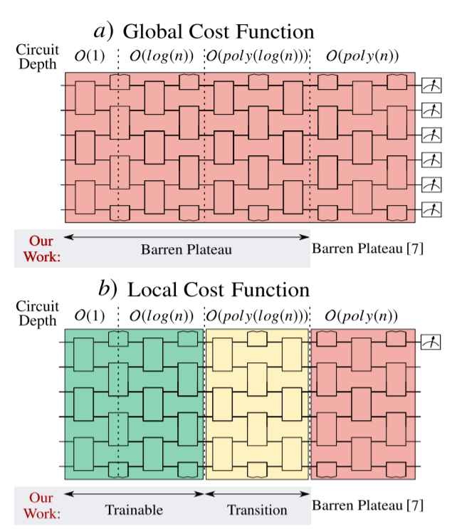
Many variational quantum algorithms are constructed to use global cost functions. Information from the entire measurement is used to analyze the result of the circuit, and a cost function is calculated from this to quantify the circuit’s performance. A local cost function only considers information from a few qubits, and attempts to analyze the behavior of the entire circuit from this limited scope.
Cerezo et al. also handily prove that these local cost functions are bounded by the global ones, i.e., if a global cost function is formulated in the manner described by Cerezo et al., then the value of its corresponding local cost function will always be less than or equal to the value of the global cost function.
In this notebook, we investigate the effect of barren plateaus in variational quantum algorithms, and how they can be mitigated using local cost functions.
We first need to import the following modules.
import pennylane as qml
from pennylane import numpy as np
import matplotlib.pyplot as plt
from matplotlib.ticker import LinearLocator, FormatStrFormatter

np.random.seed(42)
Visualizing the problem
To start, let’s look at the task of learning the identity gate across multiple qubits. This will help us visualize the problem and get a sense of what is happening in the cost landscape.
First we define a number of wires we want to train on. The work by Cerezo et al. shows that circuits are trainable under certain regimes, so how many qubits we train on will effect our results.
wires = 6
dev = qml.device("default.qubit", wires=wires, shots=10000)
Next, we want to define our QNodes and our circuit ansatz. For this simple example, an ansatz that works well is simply a rotation along X, and a rotation along Y, repeated across all the qubits.
We will also define our cost functions here. Since we are trying to learn the identity gate, a natural cost function is 1 minus the probability of measuring the zero state, denoted here as \(1 - p_{|0\rangle}\).
We will apply this across all qubits for our global cost function, i.e.,
and for the local cost function, we will sum the individual contributions from each qubit:
It might be clear to some readers now why this function can perform better. By formatting our local cost function in this way, we have essentially divided the problem up into multiple single-qubit terms, and summed all the results up.
To implement this, we will define a separate QNode for the local cost function and the global cost function.
def global_cost_simple(rotations):
    for i in range(wires):
        qml.RX(rotations[0][i], wires=i)
        qml.RY(rotations[1][i], wires=i)
    return qml.probs(wires=range(wires))

def local_cost_simple(rotations):
    for i in range(wires):
        qml.RX(rotations[0][i], wires=i)
        qml.RY(rotations[1][i], wires=i)
    return [qml.probs(wires=i) for i in range(wires)]

global_circuit = qml.QNode(global_cost_simple, dev, interface="autograd")

local_circuit = qml.QNode(local_cost_simple, dev, interface="autograd")

def cost_local(rotations):
    return 1 - np.sum([i for (i, _) in local_circuit(rotations)])/wires


def cost_global(rotations):
    return 1 - global_circuit(rotations)[0]
To analyze each of the circuits, we provide some random initial parameters for each rotation.
RX = np.random.uniform(low=-np.pi, high=np.pi)
RY = np.random.uniform(low=-np.pi, high=np.pi)
rotations = [[RX for i in range(wires)], [RY for i in range(wires)]]
Examining the results:
print("Global Cost: {: .7f}".format(cost_global(rotations)))
print("Local Cost: {: .7f}".format(cost_local(rotations)))
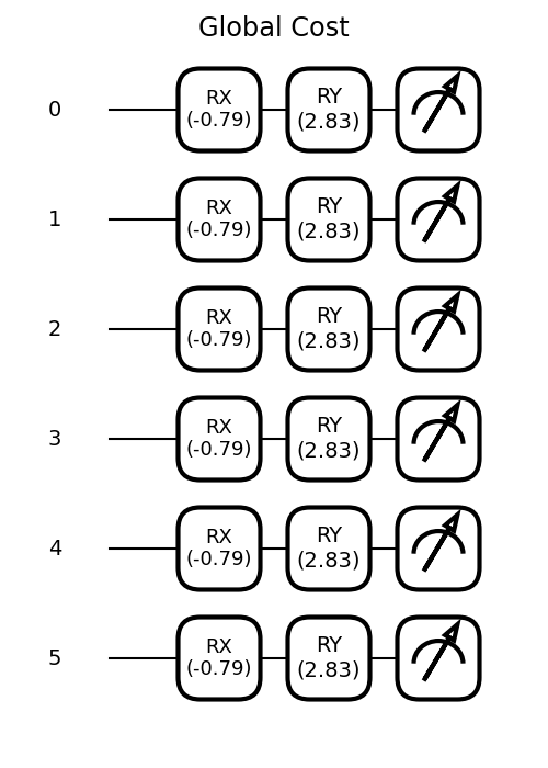
qml.drawer.use_style('black_white')
fig1, ax1 = qml.draw_mpl(global_circuit, decimals=2)(rotations)
fig1.suptitle("Global Cost", fontsize='xx-large')
plt.show()
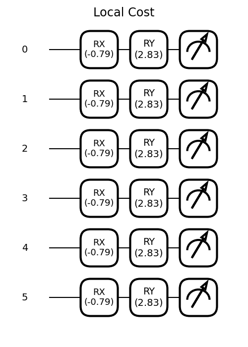
fig2, ax2 = qml.draw_mpl(local_circuit, decimals=2)(rotations)
fig2.suptitle("Local Cost", fontsize='xx-large')
plt.show()
Out:
Global Cost:  0.9999000
Local Cost:  0.8373000
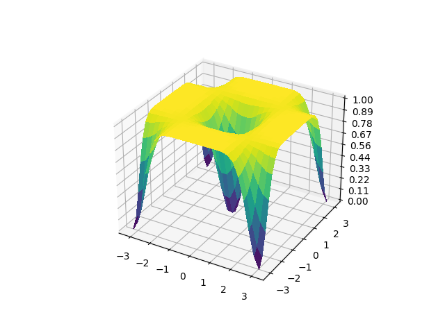
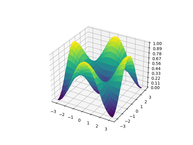
With this simple example, we can visualize the cost function, and see the barren plateau effect graphically. Although there are \(2n\) (where \(n\) is the number of qubits) parameters, in order to plot the cost landscape we must constrain ourselves. We will consider the case where all X rotations have the same value, and all the Y rotations have the same value.
Firstly, we look at the global cost function. When plotting the cost function across 6 qubits, much of the cost landscape is flat, and difficult to train (even with a circuit depth of only 2!). This effect will worsen as the number of qubits increases.
def generate_surface(cost_function):
    Z = []
    Z_assembler = []

    X = np.arange(-np.pi, np.pi, 0.25)
    Y = np.arange(-np.pi, np.pi, 0.25)
    X, Y = np.meshgrid(X, Y)

    for x in X[0, :]:
        for y in Y[:, 0]:
            rotations = [[x for i in range(wires)], [y for i in range(wires)]]
            Z_assembler.append(cost_function(rotations))
        Z.append(Z_assembler)
        Z_assembler = []

    Z = np.asarray(Z)
    return Z

def plot_surface(surface):
    X = np.arange(-np.pi, np.pi, 0.25)
    Y = np.arange(-np.pi, np.pi, 0.25)
    X, Y = np.meshgrid(X, Y)
    fig = plt.figure()
    ax = fig.add_subplot(111, projection="3d")
    surf = ax.plot_surface(X, Y, surface, cmap="viridis", linewidth=0, antialiased=False)
    ax.set_zlim(0, 1)
    ax.zaxis.set_major_locator(LinearLocator(10))
    ax.zaxis.set_major_formatter(FormatStrFormatter("%.02f"))
    plt.show()


global_surface = generate_surface(cost_global)
plot_surface(global_surface)
However, when we change to the local cost function, the cost landscape becomes much more trainable as the size of the barren plateau decreases.
local_surface = generate_surface(cost_local)
plot_surface(local_surface)

Those are some nice pictures, but how do they reflect actual trainability? Let us try training both the local and global cost functions. To simplify this model, let’s modify our cost function from
where we sum the marginal probabilities of each qubit, to
where we only consider the probability of a single qubit to be in the 0 state.
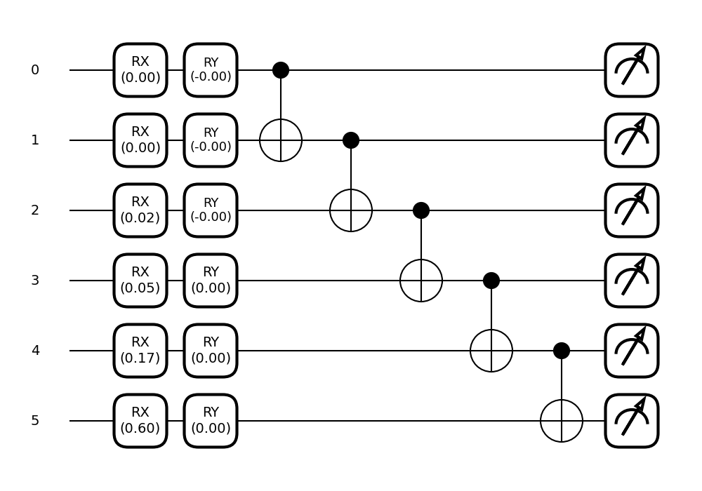
While we’re at it, let us make our ansatz a little more like one we would encounter while trying to solve a VQE problem, and add entanglement.
def global_cost_simple(rotations):
    for i in range(wires):
        qml.RX(rotations[0][i], wires=i)
        qml.RY(rotations[1][i], wires=i)
    qml.broadcast(qml.CNOT, wires=range(wires), pattern="chain")
    return qml.probs(wires=range(wires))
def local_cost_simple(rotations):
    for i in range(wires):
        qml.RX(rotations[0][i], wires=i)
        qml.RY(rotations[1][i], wires=i)
    qml.broadcast(qml.CNOT, wires=range(wires), pattern="chain")
    return qml.probs(wires=[0])

global_circuit = qml.QNode(global_cost_simple, dev, interface="autograd")

local_circuit = qml.QNode(local_cost_simple, dev, interface="autograd")

def cost_local(rotations):
    return 1 - local_circuit(rotations)[0]
def cost_global(rotations):
    return 1 - global_circuit(rotations)[0]
Of course, now that we’ve changed both our cost function and our circuit, we will need to scan the cost landscape again.
global_surface = generate_surface(cost_global)
plot_surface(global_surface)

local_surface = generate_surface(cost_local)
plot_surface(local_surface)

It seems our changes didn’t significantly alter the overall cost landscape. This probably isn’t a general trend, but it is a nice surprise. Now, let us get back to training the local and global cost functions. Because we have a visualization of the total cost landscape, let’s pick a point to exaggerate the problem. One of the worst points in the landscape is \((\pi,0)\) as it is in the middle of the plateau, so let’s use that.
rotations = np.array([[3.] * len(range(wires)), [0.] * len(range(wires))], requires_grad=True)
opt = qml.GradientDescentOptimizer(stepsize=0.2)
steps = 100
params_global = rotations
for i in range(steps):
    # update the circuit parameters
    params_global = opt.step(cost_global, params_global)

    if (i + 1) % 5 == 0:
        print("Cost after step {:5d}: {: .7f}".format(i + 1, cost_global(params_global)))
    if cost_global(params_global) < 0.1:
        break
fig, ax = qml.draw_mpl(global_circuit, decimals=2)(params_global)
plt.show()
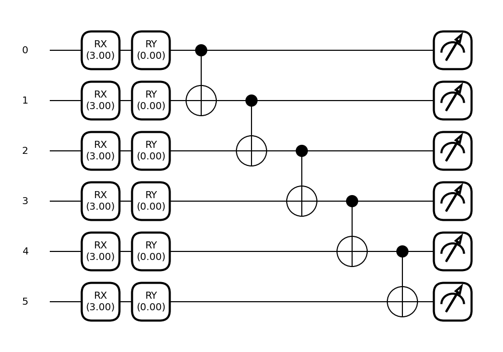
Out:
Cost after step     5:  1.0000000
Cost after step    10:  1.0000000
Cost after step    15:  1.0000000
Cost after step    20:  1.0000000
Cost after step    25:  1.0000000
Cost after step    30:  1.0000000
Cost after step    35:  1.0000000
Cost after step    40:  1.0000000
Cost after step    45:  1.0000000
Cost after step    50:  1.0000000
Cost after step    55:  1.0000000
Cost after step    60:  1.0000000
Cost after step    65:  1.0000000
Cost after step    70:  1.0000000
Cost after step    75:  1.0000000
Cost after step    80:  1.0000000
Cost after step    85:  1.0000000
Cost after step    90:  1.0000000
Cost after step    95:  1.0000000
Cost after step   100:  1.0000000
After 100 steps, the cost function is still exactly 1. Clearly we are in an “untrainable” area. Now, let us limit ourselves to the local cost function and see how it performs.
rotations = np.array([[3. for i in range(wires)], [0. for i in range(wires)]], requires_grad=True)
opt = qml.GradientDescentOptimizer(stepsize=0.2)
steps = 100
params_local = rotations
for i in range(steps):
    # update the circuit parameters
    params_local = opt.step(cost_local, params_local)

    if (i + 1) % 5 == 0:
        print("Cost after step {:5d}: {: .7f}".format(i + 1, cost_local(params_local)))
    if cost_local(params_local) < 0.05:
        break

fig, ax = qml.draw_mpl(local_circuit, decimals=2)(params_local)
plt.show()
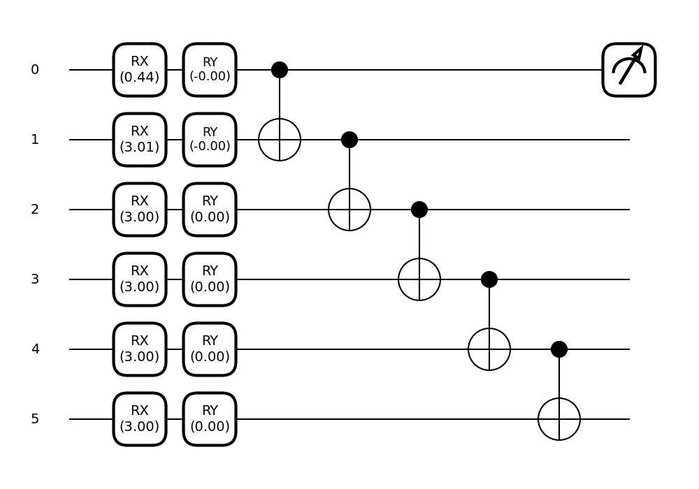
Out:
Cost after step     5:  0.9871000
Cost after step    10:  0.9651000
Cost after step    15:  0.9173000
Cost after step    20:  0.8059000
Cost after step    25:  0.6213000
Cost after step    30:  0.3703000
Cost after step    35:  0.1821000
Cost after step    40:  0.0684000
It trained! And much faster than the global case. However, we know our local cost function is bounded by the global one, but just how much have we trained it?
cost_global(params_local)
Out:
1.0
Interestingly, the global cost function is still 1. If we trained the local cost function, why hasn’t the global cost function changed?
The answer is that we have trained the global cost a little bit, but
not enough to see a change with only 10000 shots. To see the effect,
we’ll need to increase the number of shots to an unreasonable amount.
Instead, making the backend analytic by setting shots to None, gives
us the exact representation.
dev.shots = None
global_circuit = qml.QNode(global_cost_simple, dev, interface="autograd")
print(
    "Current cost: "
    + str(cost_global(params_local))
    + ".\nInitial cost: "
    + str(cost_global([[3.0 for i in range(wires)], [0 for i in range(wires)]]))
    + ".\nDifference: "
    + str(
        cost_global([[3.0 for i in range(wires)], [0 for i in range(wires)]])
        - cost_global(params_local)
    )
)
Out:
Current cost: 0.9999999999972213.
Initial cost: 0.9999999999999843.
Difference: 2.763012041384627e-12
Our circuit has definitely been trained, but not a useful amount. If we attempt to use this circuit, it would act the same as if we never trained at all. Furthermore, if we now attempt to train the global cost function, we are still firmly in the plateau region. In order to fully train the global circuit, we will need to increase the locality gradually as we train.
def tunable_cost_simple(rotations):
    for i in range(wires):
        qml.RX(rotations[0][i], wires=i)
        qml.RY(rotations[1][i], wires=i)
    qml.broadcast(qml.CNOT, wires=range(wires), pattern="chain")
    return qml.probs(range(locality))

def cost_tunable(rotations):
    return 1 - tunable_circuit(rotations)[0]

dev.shots = 10000
tunable_circuit = qml.QNode(tunable_cost_simple, dev, interface="autograd")
locality = 2
params_tunable = params_local
fig, ax = qml.draw_mpl(tunable_circuit, decimals=2)(params_tunable)
plt.show()
print(cost_tunable(params_tunable))

locality = 2
opt = qml.GradientDescentOptimizer(stepsize=0.1)
steps = 600
for i in range(steps):
    # update the circuit parameters
    params_tunable = opt.step(cost_tunable, params_tunable)

    runCost = cost_tunable(params_tunable)
    if (i + 1) % 10 == 0:
        print(
            "Cost after step {:5d}: {: .7f}".format(i + 1, runCost)
            + ". Locality: "
            + str(locality)
        )

    if runCost < 0.1 and locality < wires:
        print("---Switching Locality---")
        locality += 1
        continue
    elif runCost < 0.1 and locality >= wires:
        break
fig, ax = qml.draw_mpl(tunable_circuit, decimals=2)(params_tunable)
plt.show()
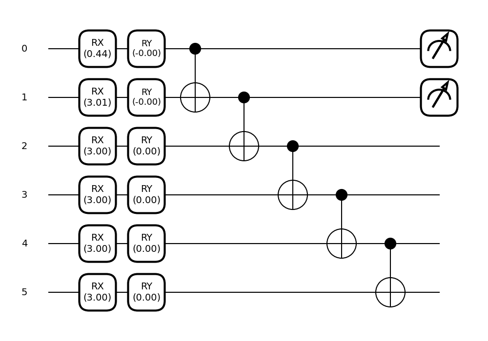
Out:
0.9957
Cost after step    10:  0.9909000. Locality: 2
Cost after step    20:  0.9753000. Locality: 2
Cost after step    30:  0.9275000. Locality: 2
Cost after step    40:  0.8386000. Locality: 2
Cost after step    50:  0.6821000. Locality: 2
Cost after step    60:  0.4353000. Locality: 2
Cost after step    70:  0.2264000. Locality: 2
Cost after step    80:  0.0923000. Locality: 2
---Switching Locality---
Cost after step    90:  0.9901000. Locality: 3
Cost after step   100:  0.9737000. Locality: 3
Cost after step   110:  0.9400000. Locality: 3
Cost after step   120:  0.8711000. Locality: 3
Cost after step   130:  0.7228000. Locality: 3
Cost after step   140:  0.5156000. Locality: 3
Cost after step   150:  0.2846000. Locality: 3
Cost after step   160:  0.1285000. Locality: 3
---Switching Locality---
Cost after step   170:  0.9899000. Locality: 4
Cost after step   180:  0.9799000. Locality: 4
Cost after step   190:  0.9512000. Locality: 4
Cost after step   200:  0.8964000. Locality: 4
Cost after step   210:  0.7683000. Locality: 4
Cost after step   220:  0.5752000. Locality: 4
Cost after step   230:  0.3314000. Locality: 4
Cost after step   240:  0.1575000. Locality: 4
---Switching Locality---
Cost after step   250:  0.9942000. Locality: 5
Cost after step   260:  0.9866000. Locality: 5
Cost after step   270:  0.9641000. Locality: 5
Cost after step   280:  0.9120000. Locality: 5
Cost after step   290:  0.8136000. Locality: 5
Cost after step   300:  0.6380000. Locality: 5
Cost after step   310:  0.4004000. Locality: 5
Cost after step   320:  0.1996000. Locality: 5
---Switching Locality---
Cost after step   330:  0.9945000. Locality: 6
Cost after step   340:  0.9873000. Locality: 6
Cost after step   350:  0.9689000. Locality: 6
Cost after step   360:  0.9288000. Locality: 6
Cost after step   370:  0.8476000. Locality: 6
Cost after step   380:  0.6711000. Locality: 6
Cost after step   390:  0.4527000. Locality: 6
Cost after step   400:  0.2342000. Locality: 6
Cost after step   410:  0.1014000. Locality: 6
A more thorough analysis
Now the circuit can be trained, even though we started from a place where the global function has a barren plateau. The significance of this is that we can now train from every starting location in this example.
But, how often does this problem occur? If we wanted to train this circuit from a random starting point, how often would we be stuck in a plateau? To investigate this, let’s attempt to train the global cost function using random starting positions and count how many times we run into a barren plateau.
Let’s use a number of qubits we are more likely to use in a real variational circuit: n=10. We will say that after 400 steps, any run with a cost function of less than 0.9 (chosen arbitrarily) will probably be trainable given more time. Any run with a greater cost function will probably be in a plateau.
This may take up to 15 minutes.
samples = 10
plateau = 0
trained = 0
opt = qml.GradientDescentOptimizer(stepsize=0.2)
steps = 400
wires = 8

dev = qml.device("default.qubit", wires=wires, shots=10000)
global_circuit = qml.QNode(global_cost_simple, dev, interface="autograd")

for runs in range(samples):
    print("--- New run! ---")
    has_been_trained = False

    params_global = np.random.uniform(-np.pi, np.pi, (2, wires), requires_grad=True)

    for i in range(steps):
        # update the circuit parameters
        params_global = opt.step(cost_global, params_global)

        if (i + 1) % 20 == 0:
            print("Cost after step {:5d}: {: .7f}".format(i + 1, cost_global(params_global)))
        if cost_global(params_global) < 0.9:
            has_been_trained = True
            break
    if has_been_trained:
        trained = trained + 1
    else:
        plateau = plateau + 1
    print("Trained: {:5d}".format(trained))
    print("Plateau'd: {:5d}".format(plateau))


samples = 10
plateau = 0
trained = 0
opt = qml.GradientDescentOptimizer(stepsize=0.2)
steps = 400
wires = 8

dev = qml.device("default.qubit", wires=wires, shots=10000)
tunable_circuit = qml.QNode(tunable_cost_simple, dev, interface="autograd")

for runs in range(samples):
    locality = 1
    print("--- New run! ---")
    has_been_trained = False

    params_tunable = np.random.uniform(-np.pi, np.pi, (2, wires), requires_grad=True)
    for i in range(steps):
        # update the circuit parameters
        params_tunable = opt.step(cost_tunable, params_tunable)

        runCost = cost_tunable(params_tunable)
        if (i + 1) % 10 == 0:
            print(
                "Cost after step {:5d}: {: .7f}".format(i + 1, runCost)
                + ". Locality: "
                + str(locality)
            )

        if runCost < 0.5 and locality < wires:
            print("---Switching Locality---")
            locality += 1
            continue
        elif runCost < 0.1 and locality >= wires:
            trained = trained + 1
            has_been_trained = True
            break
    if not has_been_trained:
        plateau = plateau + 1
    print("Trained: {:5d}".format(trained))
    print("Plateau'd: {:5d}".format(plateau))
Out:
--- New run! ---
Cost after step    20:  1.0000000
Cost after step    40:  1.0000000
Cost after step    60:  1.0000000
Cost after step    80:  1.0000000
Cost after step   100:  1.0000000
Cost after step   120:  1.0000000
Cost after step   140:  1.0000000
Cost after step   160:  1.0000000
Cost after step   180:  1.0000000
Cost after step   200:  1.0000000
Cost after step   220:  1.0000000
Cost after step   240:  1.0000000
Cost after step   260:  1.0000000
Cost after step   280:  1.0000000
Cost after step   300:  1.0000000
Cost after step   320:  1.0000000
Cost after step   340:  1.0000000
Cost after step   360:  1.0000000
Cost after step   380:  1.0000000
Cost after step   400:  1.0000000
Trained:     0
Plateau'd:     1
--- New run! ---
Cost after step    20:  0.9993000
Cost after step    40:  0.9994000
Cost after step    60:  0.9995000
Cost after step    80:  0.9994000
Cost after step   100:  0.9996000
Cost after step   120:  0.9995000
Cost after step   140:  0.9986000
Cost after step   160:  0.9993000
Cost after step   180:  0.9991000
Cost after step   200:  0.9996000
Cost after step   220:  0.9985000
Cost after step   240:  0.9989000
Cost after step   260:  0.9993000
Cost after step   280:  0.9991000
Cost after step   300:  0.9990000
Cost after step   320:  0.9987000
Cost after step   340:  0.9987000
Cost after step   360:  0.9994000
Cost after step   380:  0.9985000
Cost after step   400:  0.9991000
Trained:     0
Plateau'd:     2
--- New run! ---
Cost after step    20:  0.9976000
Cost after step    40:  0.9967000
Cost after step    60:  0.9970000
Cost after step    80:  0.9964000
Cost after step   100:  0.9956000
Cost after step   120:  0.9965000
Cost after step   140:  0.9958000
Cost after step   160:  0.9931000
Cost after step   180:  0.9940000
Cost after step   200:  0.9908000
Cost after step   220:  0.9887000
Cost after step   240:  0.9834000
Cost after step   260:  0.9821000
Cost after step   280:  0.9742000
Cost after step   300:  0.9576000
Cost after step   320:  0.9330000
Trained:     1
Plateau'd:     2
--- New run! ---
Cost after step    20:  0.9998000
Cost after step    40:  0.9997000
Cost after step    60:  0.9996000
Cost after step    80:  0.9994000
Cost after step   100:  0.9994000
Cost after step   120:  0.9996000
Cost after step   140:  0.9997000
Cost after step   160:  0.9992000
Cost after step   180:  0.9991000
Cost after step   200:  0.9992000
Cost after step   220:  0.9990000
Cost after step   240:  0.9986000
Cost after step   260:  0.9989000
Cost after step   280:  0.9988000
Cost after step   300:  0.9972000
Cost after step   320:  0.9982000
Cost after step   340:  0.9981000
Cost after step   360:  0.9979000
Cost after step   380:  0.9977000
Cost after step   400:  0.9972000
Trained:     1
Plateau'd:     3
--- New run! ---
Cost after step    20:  1.0000000
Cost after step    40:  1.0000000
Cost after step    60:  0.9999000
Cost after step    80:  1.0000000
Cost after step   100:  1.0000000
Cost after step   120:  1.0000000
Cost after step   140:  1.0000000
Cost after step   160:  0.9999000
Cost after step   180:  1.0000000
Cost after step   200:  1.0000000
Cost after step   220:  1.0000000
Cost after step   240:  1.0000000
Cost after step   260:  1.0000000
Cost after step   280:  1.0000000
Cost after step   300:  1.0000000
Cost after step   320:  1.0000000
Cost after step   340:  1.0000000
Cost after step   360:  0.9998000
Cost after step   380:  1.0000000
Cost after step   400:  1.0000000
Trained:     1
Plateau'd:     4
--- New run! ---
Cost after step    20:  0.9950000
Cost after step    40:  0.9957000
Cost after step    60:  0.9931000
Cost after step    80:  0.9920000
Cost after step   100:  0.9925000
Cost after step   120:  0.9908000
Cost after step   140:  0.9865000
Cost after step   160:  0.9861000
Cost after step   180:  0.9846000
Cost after step   200:  0.9767000
Cost after step   220:  0.9696000
Cost after step   240:  0.9560000
Cost after step   260:  0.9276000
Trained:     2
Plateau'd:     4
--- New run! ---
Cost after step    20:  0.9989000
Cost after step    40:  0.9979000
Cost after step    60:  0.9979000
Cost after step    80:  0.9982000
Cost after step   100:  0.9984000
Cost after step   120:  0.9986000
Cost after step   140:  0.9978000
Cost after step   160:  0.9976000
Cost after step   180:  0.9967000
Cost after step   200:  0.9972000
Cost after step   220:  0.9958000
Cost after step   240:  0.9966000
Cost after step   260:  0.9966000
Cost after step   280:  0.9952000
Cost after step   300:  0.9958000
Cost after step   320:  0.9972000
Cost after step   340:  0.9953000
Cost after step   360:  0.9934000
Cost after step   380:  0.9929000
Cost after step   400:  0.9916000
Trained:     2
Plateau'd:     5
--- New run! ---
Cost after step    20:  0.9988000
Cost after step    40:  0.9980000
Cost after step    60:  0.9978000
Cost after step    80:  0.9986000
Cost after step   100:  0.9978000
Cost after step   120:  0.9977000
Cost after step   140:  0.9974000
Cost after step   160:  0.9976000
Cost after step   180:  0.9975000
Cost after step   200:  0.9970000
Cost after step   220:  0.9972000
Cost after step   240:  0.9961000
Cost after step   260:  0.9960000
Cost after step   280:  0.9953000
Cost after step   300:  0.9947000
Cost after step   320:  0.9945000
Cost after step   340:  0.9912000
Cost after step   360:  0.9916000
Cost after step   380:  0.9866000
Cost after step   400:  0.9822000
Trained:     2
Plateau'd:     6
--- New run! ---
Cost after step    20:  1.0000000
Cost after step    40:  1.0000000
Cost after step    60:  1.0000000
Cost after step    80:  1.0000000
Cost after step   100:  1.0000000
Cost after step   120:  1.0000000
Cost after step   140:  1.0000000
Cost after step   160:  1.0000000
Cost after step   180:  1.0000000
Cost after step   200:  1.0000000
Cost after step   220:  1.0000000
Cost after step   240:  1.0000000
Cost after step   260:  1.0000000
Cost after step   280:  1.0000000
Cost after step   300:  1.0000000
Cost after step   320:  1.0000000
Cost after step   340:  1.0000000
Cost after step   360:  1.0000000
Cost after step   380:  1.0000000
Cost after step   400:  1.0000000
Trained:     2
Plateau'd:     7
--- New run! ---
Cost after step    20:  1.0000000
Cost after step    40:  1.0000000
Cost after step    60:  1.0000000
Cost after step    80:  1.0000000
Cost after step   100:  0.9999000
Cost after step   120:  1.0000000
Cost after step   140:  1.0000000
Cost after step   160:  1.0000000
Cost after step   180:  1.0000000
Cost after step   200:  1.0000000
Cost after step   220:  1.0000000
Cost after step   240:  1.0000000
Cost after step   260:  1.0000000
Cost after step   280:  1.0000000
Cost after step   300:  1.0000000
Cost after step   320:  1.0000000
Cost after step   340:  1.0000000
Cost after step   360:  1.0000000
Cost after step   380:  1.0000000
Cost after step   400:  1.0000000
Trained:     2
Plateau'd:     8
--- New run! ---
---Switching Locality---
Cost after step    10:  0.6137000. Locality: 2
---Switching Locality---
Cost after step    20:  0.5159000. Locality: 3
---Switching Locality---
Cost after step    30:  0.7040000. Locality: 4
Cost after step    40:  0.5823000. Locality: 4
---Switching Locality---
Cost after step    50:  0.5055000. Locality: 5
---Switching Locality---
Cost after step    60:  0.6965000. Locality: 6
Cost after step    70:  0.5823000. Locality: 6
---Switching Locality---
Cost after step    80:  0.8792000. Locality: 7
Cost after step    90:  0.7172000. Locality: 7
---Switching Locality---
Cost after step   100:  0.9741000. Locality: 8
Cost after step   110:  0.9329000. Locality: 8
Cost after step   120:  0.8278000. Locality: 8
Cost after step   130:  0.5973000. Locality: 8
Cost after step   140:  0.2649000. Locality: 8
Trained:     1
Plateau'd:     0
--- New run! ---
---Switching Locality---
Cost after step    10:  0.6273000. Locality: 2
---Switching Locality---
---Switching Locality---
Cost after step    20:  0.9218000. Locality: 4
Cost after step    30:  0.8247000. Locality: 4
Cost after step    40:  0.5992000. Locality: 4
---Switching Locality---
Cost after step    50:  0.6852000. Locality: 5
Cost after step    60:  0.6003000. Locality: 5
Cost after step    70:  0.5220000. Locality: 5
---Switching Locality---
Cost after step    80:  0.5100000. Locality: 6
---Switching Locality---
---Switching Locality---
Cost after step    90:  0.4677000. Locality: 8
Cost after step   100:  0.1562000. Locality: 8
Trained:     2
Plateau'd:     0
--- New run! ---
---Switching Locality---
---Switching Locality---
---Switching Locality---
---Switching Locality---
Cost after step    10:  0.5405000. Locality: 5
---Switching Locality---
Cost after step    20:  0.6024000. Locality: 6
---Switching Locality---
Cost after step    30:  0.6060000. Locality: 7
---Switching Locality---
Cost after step    40:  0.5009000. Locality: 8
Cost after step    50:  0.1676000. Locality: 8
Trained:     3
Plateau'd:     0
--- New run! ---
Cost after step    10:  0.4871000. Locality: 1
---Switching Locality---
Cost after step    20:  0.4948000. Locality: 2
---Switching Locality---
Cost after step    30:  0.6627000. Locality: 3
---Switching Locality---
Cost after step    40:  0.5826000. Locality: 4
---Switching Locality---
Cost after step    50:  0.5234000. Locality: 5
---Switching Locality---
---Switching Locality---
Cost after step    60:  0.6394000. Locality: 7
---Switching Locality---
Cost after step    70:  0.3126000. Locality: 8
Trained:     4
Plateau'd:     0
--- New run! ---
Cost after step    10:  0.5485000. Locality: 1
---Switching Locality---
Cost after step    20:  0.6393000. Locality: 2
---Switching Locality---
Cost after step    30:  0.8061000. Locality: 3
Cost after step    40:  0.7073000. Locality: 3
Cost after step    50:  0.6144000. Locality: 3
Cost after step    60:  0.4888000. Locality: 3
---Switching Locality---
Cost after step    70:  0.6102000. Locality: 4
---Switching Locality---
Cost after step    80:  0.4909000. Locality: 5
---Switching Locality---
Cost after step    90:  0.7897000. Locality: 6
Cost after step   100:  0.4939000. Locality: 6
---Switching Locality---
Cost after step   110:  0.7063000. Locality: 7
Cost after step   120:  0.5323000. Locality: 7
---Switching Locality---
Cost after step   130:  0.2921000. Locality: 8
Trained:     5
Plateau'd:     0
--- New run! ---
---Switching Locality---
Cost after step    10:  0.7449000. Locality: 2
Cost after step    20:  0.5005000. Locality: 2
---Switching Locality---
---Switching Locality---
---Switching Locality---
Cost after step    30:  0.7292000. Locality: 5
Cost after step    40:  0.4696000. Locality: 5
---Switching Locality---
---Switching Locality---
Cost after step    50:  0.5099000. Locality: 7
---Switching Locality---
Cost after step    60:  0.6587000. Locality: 8
Cost after step    70:  0.4912000. Locality: 8
Cost after step    80:  0.2440000. Locality: 8
Trained:     6
Plateau'd:     0
--- New run! ---
---Switching Locality---
---Switching Locality---
Cost after step    10:  0.8510000. Locality: 3
Cost after step    20:  0.7255000. Locality: 3
Cost after step    30:  0.5811000. Locality: 3
---Switching Locality---
Cost after step    40:  0.6300000. Locality: 4
---Switching Locality---
Cost after step    50:  0.8801000. Locality: 5
Cost after step    60:  0.7395000. Locality: 5
---Switching Locality---
Cost after step    70:  0.8948000. Locality: 6
Cost after step    80:  0.7399000. Locality: 6
---Switching Locality---
Cost after step    90:  0.7139000. Locality: 7
Cost after step   100:  0.5959000. Locality: 7
---Switching Locality---
Cost after step   110:  0.5939000. Locality: 8
Cost after step   120:  0.2906000. Locality: 8
Trained:     7
Plateau'd:     0
--- New run! ---
---Switching Locality---
Cost after step    10:  0.6986000. Locality: 2
Cost after step    20:  0.6273000. Locality: 2
Cost after step    30:  0.5645000. Locality: 2
Cost after step    40:  0.5016000. Locality: 2
---Switching Locality---
Cost after step    50:  0.9048000. Locality: 3
Cost after step    60:  0.7903000. Locality: 3
Cost after step    70:  0.5948000. Locality: 3
---Switching Locality---
---Switching Locality---
Cost after step    80:  0.5600000. Locality: 5
---Switching Locality---
Cost after step    90:  0.8307000. Locality: 6
Cost after step   100:  0.6442000. Locality: 6
---Switching Locality---
Cost after step   110:  0.7075000. Locality: 7
Cost after step   120:  0.5936000. Locality: 7
---Switching Locality---
Cost after step   130:  0.7649000. Locality: 8
Cost after step   140:  0.6810000. Locality: 8
Cost after step   150:  0.5936000. Locality: 8
Cost after step   160:  0.4526000. Locality: 8
Cost after step   170:  0.1974000. Locality: 8
Trained:     8
Plateau'd:     0
--- New run! ---
Cost after step    10:  0.5488000. Locality: 1
---Switching Locality---
Cost after step    20:  0.8358000. Locality: 2
Cost after step    30:  0.7614000. Locality: 2
Cost after step    40:  0.6718000. Locality: 2
Cost after step    50:  0.4921000. Locality: 2
---Switching Locality---
---Switching Locality---
Cost after step    60:  0.6433000. Locality: 4
---Switching Locality---
Cost after step    70:  0.7787000. Locality: 5
Cost after step    80:  0.5250000. Locality: 5
---Switching Locality---
Cost after step    90:  0.5270000. Locality: 6
---Switching Locality---
---Switching Locality---
Cost after step   100:  0.9690000. Locality: 8
Cost after step   110:  0.9106000. Locality: 8
Cost after step   120:  0.7561000. Locality: 8
Cost after step   130:  0.4537000. Locality: 8
Cost after step   140:  0.1197000. Locality: 8
Trained:     9
Plateau'd:     0
--- New run! ---
---Switching Locality---
Cost after step    10:  0.6759000. Locality: 2
---Switching Locality---
Cost after step    20:  0.8020000. Locality: 3
Cost after step    30:  0.6412000. Locality: 3
---Switching Locality---
Cost after step    40:  0.6920000. Locality: 4
---Switching Locality---
Cost after step    50:  0.7176000. Locality: 5
Cost after step    60:  0.5973000. Locality: 5
---Switching Locality---
Cost after step    70:  0.5469000. Locality: 6
---Switching Locality---
Cost after step    80:  0.7019000. Locality: 7
Cost after step    90:  0.6006000. Locality: 7
---Switching Locality---
Cost after step   100:  0.8612000. Locality: 8
Cost after step   110:  0.7023000. Locality: 8
Cost after step   120:  0.4108000. Locality: 8
Cost after step   130:  0.1081000. Locality: 8
Trained:    10
Plateau'd:     0
In the global case, anywhere between 70-80% of starting positions are untrainable, a significant number. It is likely that, as the complexity of our ansatz—and the number of qubits—increases, this factor will increase.
We can compare that to our local cost function, where every single area trained, and most even trained in less time. While these examples are simple, this local-vs-global cost behaviour has been shown to extend to more complex problems.
References
- 1(1,2)
Cerezo, M., Sone, A., Volkoff, T., Cincio, L., and Coles, P. (2020). Cost-Function-Dependent Barren Plateaus in Shallow Quantum Neural Networks. arXiv:2001.00550