Optimization using SPSA

Authors: Antal Szava & David Wierichs — Posted: 19 March 2021. Last updated: 23 February 2023.

In this tutorial, we investigate using a stochastic optimizer called the Simultaneous Perturbation Stochastic Approximation (SPSA) algorithm to optimize quantum circuits. This optimizer is built into PennyLane as SPSAOptimizer. SPSA is a technique that involves approximating the gradient of a quantum circuit without having to compute it exactly.

This demonstration shows how the SPSA optimizer performs on the following tasks, compared to a gradient descent optimization:

1. A simple task on a sampling device,

2. The variational quantum eigensolver on a simulated hardware device.

Throughout the demo, we show results obtained with SPSA and with gradient descent and also compare the number of executed circuits required to complete each optimization.

Background

In PennyLane, quantum gradients on hardware are commonly computed using parameter-shift rules. Computing quantum gradients involves evaluating the partial derivative of the quantum function with respect to every free parameter. These partial derivatives are then used to apply the chain rule to compute the gradient of the quantum circuit. For qubit operations that are generated by one of the Pauli matrices, each partial derivative computation will involve two quantum circuit evaluations with a positive and a negative shift in the parameter values.

As there are two circuit evaluations for each free parameter, the number of overall quantum circuit executions for computing a quantum gradient can be expected to scale as \(O(p)\) with the number of free parameters \(p\). This scaling can be very costly for optimization tasks with many free parameters. For the overall optimization this scaling means we need \(O(pn)\) quantum circuit evaluations, where \(n\) is the number of optimization steps taken.

Fortunately, there are certain optimization techniques that offer an alternative to computing the gradients of quantum circuits. One such technique is called the Simultaneous Perturbation Stochastic Approximation (SPSA) algorithm 1. SPSA is an optimization method that involves approximating the gradient of the cost function at each iteration step. This technique requires only two quantum circuit executions per iteration step, regardless of the number of free parameters. Therefore the overall number of circuit executions would be \(O(n')\) where \(n'\) is the number of optimization steps taken when using SPSA. This technique is also considered robust against noise, making it a great optimization method in the NISQ era.

In this demo, you’ll learn how the SPSA algorithm works, and how to apply it in PennyLane to compute gradients of quantum circuits. You’ll also see it in action using noisy quantum data!

Simultaneous perturbation stochastic approximation (SPSA)

SPSA is a general method for minimizing differentiable multivariate functions. It is particularly useful for functions for which evaluating the gradient is not possible, or too resource intensive. SPSA provides a stochastic method for approximating the gradient of the cost function. To accomplish this, the cost function is evaluated twice using perturbed parameter vectors: every component of the original parameter vector is simultaneously shifted with a randomly generated value. This is in contrast to finite-differences methods where for each evaluation only one component of the parameter vector is shifted at a time.

Similar to gradient-based approaches such as gradient descent, SPSA is an iterative optimization algorithm. Let’s consider a differentiable cost function \(L(\theta)\) where \(\theta\) is a \(p\)-dimensional vector and where the optimization problem can be translated into finding a optimal parameter setting \(\theta^*\) at which \(\frac{\partial L}{\partial \theta} = 0\). It is assumed that measurements of \(L(\theta)\) are available at various values of \(\theta\)—this is exactly the problem that we’d consider when optimizing quantum functions!

SPSA starts with an initial parameter vector \(\hat{\theta}_{0}\). Its update rule is very similar to the one of standard gradient descent:

\[\hat{\theta}_{k+1} = \hat{\theta}_{k} - a_{k}\hat{g}_{k}(\hat{\theta}_{k}),\]

where \(\hat{g}_{k}\) is the stochastic estimate of the gradient \(g(\theta) = \frac{ \partial L}{\partial \theta}\) at the iterate \(\hat{\theta}_{k}\) based on prior measurements of the cost function, and \(a_{k}\) is a positive number 1.

One of the advantages of SPSA is that it is robust to noise that may occur when measuring the function \(L\). Therefore, let’s consider the function \(y(\theta)=L(\theta) + \varepsilon\), where \(\varepsilon\) is some perturbation of the output. In SPSA, the estimated gradient at each iteration step is expressed as

\[\hat{g}_{ki} (\hat{\theta}_{k}) = \frac{y(\hat{\theta}_{k} +c_{k}\Delta_{k}) - y(\hat{\theta}_{k} -c_{k}\Delta_{k})}{2c_{k}\Delta_{ki}},\]

where \(c_{k}\) is a positive number and \(\Delta_{k} = (\Delta_{k_1}, \Delta_{k_2}, ..., \Delta_{k_p})^{T}\) is a perturbation vector. The stochasticity of the technique comes from the fact that for each iteration step \(k\) the components of the \(\Delta_{k}\) perturbation vector are randomly generated using a zero-mean distribution. In most cases, the Rademacher distribution is used, meaning each parameter is simultaneously perturbed by either \(\pm c_k\).

It is this perturbation that makes SPSA robust to noise — since every parameter is already being shifted, additional shifts due to noise are less likely to hinder the optimization process. In a sense, noise gets “absorbed” into the already-stochastic process. This is highlighted in the figure below, which portrays an example of the type of path SPSA takes through the space of the function, compared to a standard gradient-based optimizer.

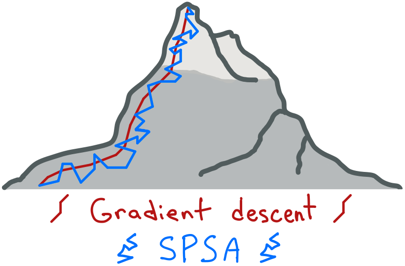
A schematic of the search paths used by gradient descent with parameter-shift and SPSA.

Now that we have explored how SPSA works, let’s see how it performs in practice!

Optimization on a sampling device

First, let’s consider a simple quantum circuit on a sampling device. For this, we’ll be using a device from the PennyLane-Qiskit plugin that samples quantum circuits to get measurement outcomes and later post-processes these outcomes to compute statistics like expectation values.

Note

Just as with other PennyLane device, the number of samples taken for a circuit execution can be specified using the shots keyword argument of the device.

Once we have a device selected, we just need a couple of other ingredients for the pieces of an example optimization to come together:

• a circuit ansatz: StronglyEntanglingLayers(),

• initial parameters: the correct shape can be computed by the shape method of the ansatz. We also use a seed so that we can simulate the same optimization every time (except for the device noise and shot noise).

• an observable: \(\bigotimes_{i=0}^{N-1}\sigma_z^i\), where \(N\) stands for the number of qubits.

• the number of layers in the ansatz and the number of wires. We choose five layers and four wires.

import pennylane as qml
from pennylane import numpy as np

num_wires = 4
num_layers = 5

device = qml.device("qiskit.aer", wires=num_wires, shots=1000)

ansatz = qml.StronglyEntanglingLayers

all_pauliz_tensor_prod = qml.prod(*[qml.PauliZ(i) for i in range(num_wires)])


def circuit(param):
    ansatz(param, wires=list(range(num_wires)))
    return qml.expval(all_pauliz_tensor_prod)


cost_function = qml.QNode(circuit, device)

np.random.seed(50)

param_shape = ansatz.shape(num_layers, num_wires)
init_param = np.random.normal(scale=0.1, size=param_shape, requires_grad=True)

We will execute a few optimizations in this demo, so let’s prepare a convenience function that runs an optimizer instance and records the cost values along the way. Together with the number of executed circuits, this will be an interesting quantity to evaluate the optimization cost on hardware!

def run_optimizer(opt, cost_function, init_param, num_steps, interval, execs_per_step):
    # Copy the initial parameters to make sure they are never overwritten
    param = init_param.copy()

    # Obtain the device used in the cost function
    dev = cost_function.device

    # Initialize the memory for cost values during the optimization
    cost_history = []
    # Monitor the initial cost value
    cost_history.append(cost_function(param))
    exec_history = [0]

    print(f"\nRunning the {opt.__class__.__name__} optimizer for {num_steps} iterations.")
    for step in range(num_steps):
        # Print out the status of the optimization
        if step % interval == 0:
            print(
                f"Step {step:3d}: Circuit executions: {exec_history[step]:4d}, "
                f"Cost = {cost_history[step]}"
            )

        # Perform an update step
        param = opt.step(cost_function, param)

        # Monitor the cost value
        cost_history.append(cost_function(param))
        exec_history.append((step + 1) * execs_per_step)

    print(
        f"Step {num_steps:3d}: Circuit executions: {exec_history[-1]:4d}, "
        f"Cost = {cost_history[-1]}"
    )
    return cost_history, exec_history

Once we have defined each piece of the optimization, there’s only one remaining component required: the SPSA optimizer. We’ll use the SPSAOptimizer built into PennyLane, for 200 iterations in total.

Choosing the hyperparameters

The SPSAOptimizer allows us to choose the initial value of two hyperparameters for SPSA: the \(c\) and \(a\) coefficients. Recall from above that the \(c\) values control the scale of the random shifts when evaluating the cost function, while the \(a\) coefficient is analogous to a learning rate and affects the rate at which the parameters change at each update step.

With stochastic approximation, specifying such hyperparameters significantly influences the convergence of the optimization for a given problem. Although there is no universal recipe for selecting these values (as they depend strongly on the specific problem), 2 includes guidelines for the selection. In our case, the initial values for \(c\) and \(a\) were selected as a result of a grid search to ensure a fast convergence. We further note that apart from \(c\) and \(a\), there are further coefficients that are initialized in the SPSAOptimizer using the previously mentioned guidelines. For more details, also consider the PennyLane documentation of the optimizer

num_steps_spsa = 200
opt = qml.SPSAOptimizer(maxiter=num_steps_spsa, c=0.15, a=0.2)
# We spend 2 circuit evaluations per step:
execs_per_step = 2
cost_history_spsa, exec_history_spsa = run_optimizer(
    opt, cost_function, init_param, num_steps_spsa, 20, execs_per_step
)

Out:

Running the SPSAOptimizer optimizer for 200 iterations.
Step   0: Circuit executions:    0, Cost = 0.902
Step  20: Circuit executions:   40, Cost = 0.276
Step  40: Circuit executions:   80, Cost = -0.732
Step  60: Circuit executions:  120, Cost = -0.894
Step  80: Circuit executions:  160, Cost = -0.962
Step 100: Circuit executions:  200, Cost = -0.98
Step 120: Circuit executions:  240, Cost = -0.972
Step 140: Circuit executions:  280, Cost = -0.994
Step 160: Circuit executions:  320, Cost = -0.982
Step 180: Circuit executions:  360, Cost = -0.99
Step 200: Circuit executions:  400, Cost = -0.994

Now let’s perform the same optimization using gradient descent. We set the step size according to a favourable value found after grid search for fast convergence.

num_steps_grad = 15
opt = qml.GradientDescentOptimizer(stepsize=0.3)
# We spend 2 circuit evaluations per parameter per step:
execs_per_step = 2 * np.prod(param_shape)
cost_history_grad, exec_history_grad = run_optimizer(
    opt, cost_function, init_param, num_steps_grad, 3, execs_per_step
)

Out:

Running the GradientDescentOptimizer optimizer for 15 iterations.
Step   0: Circuit executions:    0, Cost = 0.914
Step   3: Circuit executions:  360, Cost = -0.414
Step   6: Circuit executions:  720, Cost = -0.994
Step   9: Circuit executions: 1080, Cost = -0.998
Step  12: Circuit executions: 1440, Cost = -0.996
Step  15: Circuit executions: 1800, Cost = -0.994

SPSA and gradient descent comparison

At this point, nothing else remains but to check which of these approaches did better!

import matplotlib.pyplot as plt

plt.figure(figsize=(10, 6))

plt.plot(exec_history_grad, cost_history_grad, label="Gradient descent")
plt.plot(exec_history_spsa, cost_history_spsa, label="SPSA")

plt.xlabel("Circuit executions", fontsize=14)
plt.ylabel("Cost function value", fontsize=14)
plt.grid()

plt.title("Gradient descent vs. SPSA for simple optimization", fontsize=16)
plt.legend(fontsize=14)
plt.show()

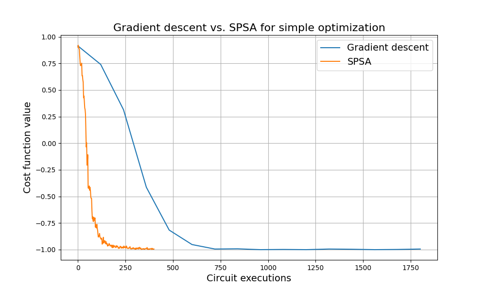
It seems that SPSA performs great and it does so with significant savings when compared to gradient descent!

Let’s take a deeper dive to see how much better it actually is by computing the ratio of required circuit executions to reach an absolute accuracy of 0.01.

grad_execs_to_prec = exec_history_grad[np.where(np.array(cost_history_grad) < -0.99)[0][0]]
spsa_execs_to_prec = exec_history_spsa[np.where(np.array(cost_history_spsa) < -0.99)[0][0]]
print(f"Circuit execution ratio: {np.round(grad_execs_to_prec/spsa_execs_to_prec, 3)}.")

Out:

Circuit execution ratio: 2.59.

This means that SPSA found the minimum up to an absolute accuracy of 0.01 while using multiple times fewer circuit executions than gradient descent! That’s an important saving, especially when running the algorithm on actual quantum hardware.

SPSA and the variational quantum eigensolver

Now that we’ve explored the theoretical underpinnings of SPSA and its use for a toy problem optimization, let’s use it to optimize a real chemical system, namely that of the hydrogen molecule \(H_2\). This molecule was studied previously in the introductory variational quantum eigensolver (VQE) demo, and so we will reuse some of that machinery below to set up the problem.

The \(H_2\) Hamiltonian uses 4 qubits, contains 15 terms, and has a ground state energy of \(-1.136189454088\) Hartree.

from pennylane import qchem

symbols = ["H", "H"]
coordinates = np.array([0.0, 0.0, -0.6614, 0.0, 0.0, 0.6614])
h2_ham, num_qubits = qchem.molecular_hamiltonian(symbols, coordinates)
h2_ham = qml.Hamiltonian(qml.math.real(h2_ham.coeffs), h2_ham.ops)

true_energy = -1.136189454088


# Variational ansatz for H_2 - see Intro VQE demo for more details
def ansatz(param, wires):
    qml.BasisState(np.array([1, 1, 0, 0]), wires=wires)
    for i in wires:
        qml.Rot(*param[0, i], wires=i)
    qml.CNOT(wires=[2, 3])
    qml.CNOT(wires=[2, 0])
    qml.CNOT(wires=[3, 1])
    for i in wires:
        qml.Rot(*param[1, i], wires=i)

Since SPSA is robust to noise, let’s see how it fares compared to gradient descent when run on noisy hardware. For this, we will set up and use a simulated version of IBM Q’s hardware.

# Note: you will need to be authenticated to IBMQ to run the following (commented) code.
# Do not run the simulation on this device, as it will send it to real hardware
# For access to IBMQ, the following statements will be useful:
# from qiskit import IBMQ
# IBMQ.load_account() # Load account from disk
# List the providers to pick an available backend:
# IBMQ.providers()    # List all available providers
# dev = qml.device("qiskit.ibmq", wires=num_qubits, backend="ibmq_lima")

from qiskit.providers.aer import noise
from qiskit.providers.fake_provider import FakeLima

# Load a fake backed to create a noise model, and create a device using that model
noise_model = noise.NoiseModel.from_backend(FakeLima())
noisy_device = qml.device(
    "qiskit.aer", wires=num_qubits, shots=1000, noise_model=noise_model
)


def circuit(param):
    ansatz(param, range(num_qubits))
    return qml.expval(h2_ham)


cost_function = qml.QNode(circuit, noisy_device)

# This random seed was used in the original VQE demo and is known to allow the
# gradient descent algorithm to converge to the global minimum.
np.random.seed(0)
param_shape = (2, num_qubits, 3)
init_param = np.random.normal(0, np.pi, param_shape, requires_grad=True)

# Initialize the optimizer - optimal step size was found through a grid search
opt = qml.GradientDescentOptimizer(stepsize=2.2)

# We spend 2 * 15 circuit evaluations per parameter per step, as there are
# 15 Hamiltonian terms
execs_per_step = 2 * 15 * np.prod(param_shape)
# Run the optimization
cost_history_grad, exec_history_grad = run_optimizer(
    opt, cost_function, init_param, num_steps_grad, 3, execs_per_step
)

final_energy = cost_history_grad[-1]
print(f"\nFinal estimated value of the ground state energy = {final_energy:.8f} Ha")
print(
    f"Distance to the true ground state energy: {np.abs(final_energy - true_energy):.8f} Ha"
)

Out:

Running the GradientDescentOptimizer optimizer for 15 iterations.
Step   0: Circuit executions:    0, Cost = 0.3718752190579573
Step   3: Circuit executions: 2160, Cost = -0.4901567596835819
Step   6: Circuit executions: 4320, Cost = -0.9669698574468821
Step   9: Circuit executions: 6480, Cost = -1.0403394706302322
Step  12: Circuit executions: 8640, Cost = -1.0453833187481136
Step  15: Circuit executions: 10800, Cost = -1.0449415367845136

Final estimated value of the ground state energy = -1.04494154 Ha
Distance to the true ground state energy: 0.09124792 Ha

What does the optimization with gradient descent look like? Let’s plot the energy during optimization and compare it to the exact ground state energy of the molecule:

plt.figure(figsize=(10, 6))

plt.plot(exec_history_grad, cost_history_grad, label="Gradient descent")

plt.xticks(fontsize=13)
plt.yticks(fontsize=13)
plt.xlabel("Circuit executions", fontsize=14)
plt.ylabel("Energy (Ha)", fontsize=14)
plt.grid()

plt.axhline(y=true_energy, color="black", linestyle="--", label="True energy")

plt.legend(fontsize=14)

plt.title("H2 energy from VQE with gradient descent", fontsize=16)

plt.show()

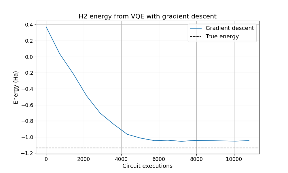
On noisy hardware, the energy never quite reaches its true value, no matter how many iterations are used. This is due to the noise as well as the stochastic nature of quantum measurements and the way they are realized on hardware. The simulator of the noisy quantum device allows us to observe these features.

VQE with SPSA

Now let’s perform the same experiment using SPSA for the VQE optimization. SPSA should use only 2 circuit executions per term in the expectation value. Since there are 15 terms and we choose 160 iterations with two evaluations for each gradient estimate, we expect 4800 total device executions.

num_steps_spsa = 160
opt = qml.SPSAOptimizer(maxiter=num_steps_spsa, c=0.3, a=1.5)

# We spend 2 * 15 circuit evaluations per step, as there are 15 Hamiltonian terms
execs_per_step = 2 * 15
# Run the optimization
cost_history_spsa, exec_history_spsa = run_optimizer(
    opt, cost_function, init_param, num_steps_spsa, 20, execs_per_step
)
final_energy = cost_history_spsa[-1]

print(f"\nFinal estimated value of the ground state energy = {final_energy:.8f} Ha")
print(
    f"Distance to the true ground state energy: {np.abs(final_energy - true_energy):.8f} Ha"
)

Out:

Running the SPSAOptimizer optimizer for 160 iterations.
Step   0: Circuit executions:    0, Cost = 0.34509355028278027
Step  20: Circuit executions:  600, Cost = -0.21453595982625445
Step  40: Circuit executions: 1200, Cost = -0.6410239342341741
Step  60: Circuit executions: 1800, Cost = -0.9070725982476936
Step  80: Circuit executions: 2400, Cost = -1.0228845251347884
Step 100: Circuit executions: 3000, Cost = -1.043082658269784
Step 120: Circuit executions: 3600, Cost = -1.0389725620169656
Step 140: Circuit executions: 4200, Cost = -1.053707617421551
Step 160: Circuit executions: 4800, Cost = -1.0492607620062273

Final estimated value of the ground state energy = -1.04926076 Ha
Distance to the true ground state energy: 0.08692869 Ha

The SPSA optimization seems to have found a similar energy value. We again take a look at how the optimization curves compare, in particular with respect to the circuit executions spent on the task.

plt.figure(figsize=(10, 6))

plt.plot(exec_history_grad, cost_history_grad, label="Gradient descent")
plt.plot(exec_history_spsa, cost_history_spsa, label="SPSA")
plt.axhline(y=true_energy, color="black", linestyle="--", label="True energy")

plt.title("$H_2$ energy from VQE using gradient descent vs. SPSA", fontsize=16)
plt.xlabel("Circuit executions", fontsize=14)
plt.ylabel("Energy (Ha)", fontsize=14)
plt.grid()

plt.legend(fontsize=14)
plt.show()

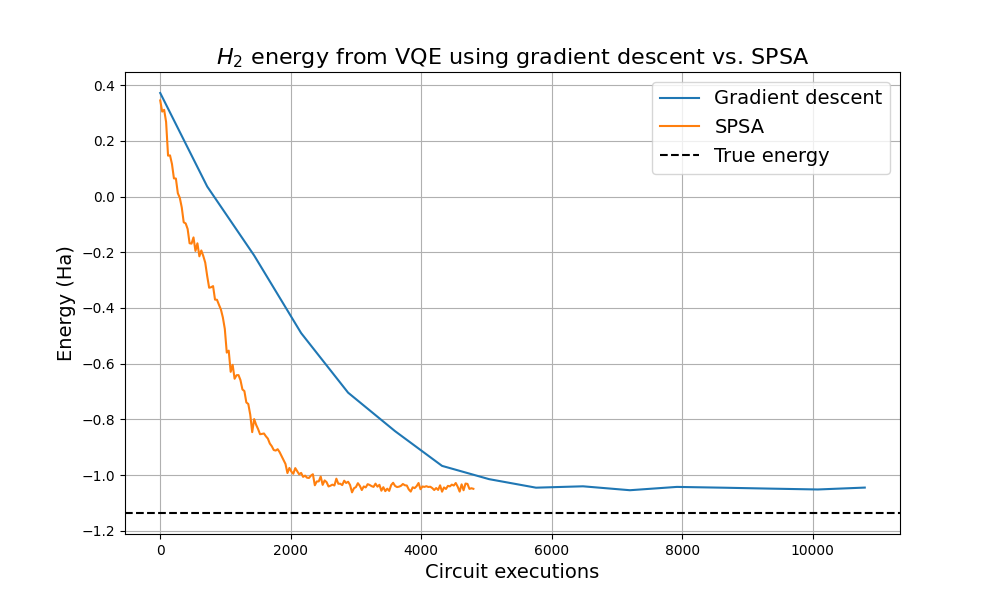
We observe here that the SPSA optimizer again converges in fewer device executions than the gradient descent optimizer. 🎉

Due to the (simulated) hardware noise, however, the obtained energies are higher than the true ground state energy. In addition, the output still bounces around, which is due to shot noise and the inherently stochastic nature of SPSA.

Conclusion

SPSA is a useful optimization technique that may be particularly beneficial on near-term quantum hardware. It uses significantly fewer circuit executions to achieve comparable results as gradient-based methods, giving it the potential to save time and resources. It can be a good alternative to gradient-based methods when the optimization problem involves executing quantum circuits with many free parameters.

There are also extensions to SPSA that could be interesting to explore in this context. One, in particular, uses an adaptive technique to approximate the Hessian matrix during optimization to effectively increase the convergence rate of SPSA 3.

In addition, there is a proposal to use an SPSA variant of the quantum natural gradient 4. This is implemented in PennyLane as well and we discuss it in the demo on QNSPSA.

References

1(1,2)

James C. Spall, “An Overview of the Simultaneous Perturbation Method for Efficient Optimization”, 1998

2

J. C. Spall, “Implementation of the simultaneous perturbation algorithm for stochastic optimization,” in IEEE Transactions on Aerospace and Electronic Systems, vol. 34, no. 3, pp. 817-823, July 1998, doi: 10.1109/7.705889.

3

J. C. Spall, “Adaptive stochastic approximation by the simultaneous perturbation method,” in IEEE Transactions on Automatic Control, vol. 45, no. 10, pp. 1839-1853, Oct 2020, doi: 10.1109/TAC.2000.880982.

4

J. Gacon, C. Zoufal, G. Carleo, and S. Woerner “Simultaneous Perturbation Stochastic Approximation of the Quantum Fisher Information”, Quantum, 5, 567, Oct 2021

About the author

Antal Szava

Antal is a senior quantum software developer at Xanadu working on PennyLane. In his spare time he enjoys watching TV shows, being active outside with friends and learning about acting.

David Wierichs

David is a researcher and quantum software developer at Xanadu, who likes to think about quantum gradients and how to use them in variational quantum algorithms. He enjoys sharing ideas in science and open source software and likes implementing cool stuff in PennyLane.

demos/tutorial_spsa

 

Download Python script

 

Download Notebook

 

View on GitHub