The Quantum Graph Recurrent Neural Network

Author: Jack Ceroni — Posted: 27 July 2020. Last updated: 25 March 2021.

This demonstration investigates quantum graph recurrent neural networks (QGRNN), which are the quantum analogue of a classical graph recurrent neural network, and a subclass of the more general quantum graph neural network ansatz. Both the QGNN and QGRNN were introduced in this paper (2019).

The Idea

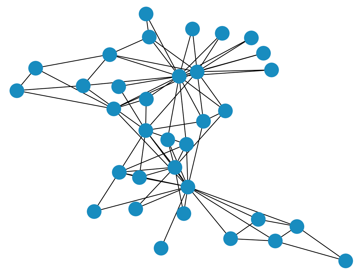
A graph is defined as a set of nodes along with a set of edges, which represent connections between nodes. Information can be encoded into graphs by assigning numbers to nodes and edges, which we call weights. It is usually convenient to think of a graph visually:

In recent years, the concept of a graph neural network (GNN) has been receiving a lot of attention from the machine learning community. A GNN seeks to learn a representation (a mapping of data into a low-dimensional vector space) of a given graph with feature vectors assigned to nodes and edges. Each of the vectors in the learned representation preserves not only the features, but also the overall topology of the graph, i.e., which nodes are connected by edges. The quantum graph neural network attempts to do something similar, but for features that are quantum-mechanical; for instance, a collection of quantum states.

Consider the class of qubit Hamiltonians that are quadratic, meaning that the terms of the Hamiltonian represent either interactions between two qubits, or the energy of individual qubits. This class of Hamiltonians is naturally described by graphs, with second-order terms between qubits corresponding to weighted edges between nodes, and first-order terms corresponding to node weights.

A well known example of a quadratic Hamiltonian is the transverse-field Ising model, which is defined as

\[\hat{H}_{\text{Ising}}(\boldsymbol\theta) \ = \ \displaystyle\sum_{(i, j) \in E} \theta_{ij}^{(1)} Z_{i} Z_{j} \ + \ \displaystyle\sum_{i} \theta_{i}^{(2)} Z_{i} \ + \ \displaystyle\sum_{i} X_{i},\]

where \(\boldsymbol\theta \ = \ \{\theta^{(1)}, \ \theta^{(2)}\}\). In this Hamiltonian, the set \(E\) that determines which pairs of qubits have \(ZZ\) interactions can be represented by the set of edges for some graph. With the qubits as nodes, this graph is called the interaction graph. The \(\theta^{(1)}\) parameters correspond to the edge weights and the \(\theta^{(2)}\) parameters correspond to weights on the nodes.

This result implies that we can think about quantum circuits with graph-theoretic properties. Recall that the time-evolution operator with respect to some Hamiltonian \(H\) is defined as:

\[U \ = \ e^{-it H}.\]

Thus, we have a clean way of taking quadratic Hamiltonians and turning them into unitaries (quantum circuits) that preserve the same correspondance to a graph. In the case of the Ising Hamiltonian, we have:

\[U_{\text{Ising}} \ = \ e^{-it \hat{H}_{\text{Ising}} (\boldsymbol\theta)} \ = \ \exp \Big[ -it \Big( \displaystyle\sum_{(i, j) \in E} \theta_{ij}^{(1)} Z_{i} Z_{j} \ + \ \displaystyle\sum_{i} \theta_{i}^{(2)} Z_{i} \ + \ \displaystyle\sum_{i} X_{i} \Big) \Big]\]

In general, this kind of unitary is very difficult to implement on a quantum computer. However, we can approximate it using the Trotter-Suzuki decomposition:

\[\exp \Big[ -it \Big( \displaystyle\sum_{(i, j) \in E} \theta_{ij}^{(1)} Z_{i} Z_{j} \ + \ \displaystyle\sum_{i} \theta_{i}^{(2)} Z_{i} \ + \ \displaystyle\sum_{i} X_{i} \Big) \Big] \ \approx \ \displaystyle\prod_{k \ = \ 1}^{t / \Delta} \Bigg[ \displaystyle\prod_{j \ = \ 1}^{Q} e^{-i \Delta \hat{H}_{\text{Ising}}^{j}(\boldsymbol\theta)} \Bigg]\]

where \(\hat{H}_{\text{Ising}}^{j}(\boldsymbol\theta)\) is the \(j\)-th term of the Ising Hamiltonian and \(\Delta\) is some small number.

This circuit is a specific instance of the Quantum Graph Recurrent Neural Network, which in general is defined as a variational ansatz of the form

\[U_{H}(\boldsymbol\mu, \ \boldsymbol\gamma) \ = \ \displaystyle\prod_{i \ = \ 1}^{P} \Bigg[ \displaystyle\prod_{j \ = \ 1}^{Q} e^{-i \gamma_j H^{j}(\boldsymbol\mu)} \Bigg],\]

for some parametrized quadratic Hamiltonian, \(H(\boldsymbol\mu)\).

Using the QGRNN

Since the QGRNN ansatz is equivalent to the approximate time evolution of some quadratic Hamiltonian, we can use it to learn the dynamics of a quantum system.

Continuing with the Ising model example, let’s imagine we have some system governed by \(\hat{H}_{\text{Ising}}(\boldsymbol\alpha)\) for an unknown set of target parameters, \(\boldsymbol\alpha\) and an unknown interaction graph \(G\). Let’s also suppose we have access to copies of some low-energy, non-ground state of the target Hamiltonian, \(|\psi_0\rangle\). In addition, we have access to a collection of time-evolved states, \(\{ |\psi(t_1)\rangle, \ |\psi(t_2)\rangle, \ ..., \ |\psi(t_N)\rangle \}\), defined by:

\[|\psi(t_k)\rangle \ = \ e^{-i t_k \hat{H}_{\text{Ising}}(\boldsymbol\alpha)} |\psi_0\rangle.\]

We call the low-energy states and the collection of time-evolved states quantum data. From here, we randomly pick a number of time-evolved states from our collection. For any state that we choose, which is evolved to some time \(t_k\), we compare it to

\[U_{\hat{H}_{\text{Ising}}}(\boldsymbol\mu, \ \Delta) |\psi_0\rangle \ \approx \ e^{-i t_k \hat{H}_{\text{Ising}}(\boldsymbol\mu)} |\psi_0\rangle.\]

This is done by feeding one of the copies of \(|\psi_0\rangle\) into a quantum circuit with the QGRNN ansatz, with some guessed set of parameters \(\boldsymbol\mu\) and a guessed interaction graph, \(G'\). We then use a classical optimizer to maximize the average “similarity” between the time-evolved states and the states prepared with the QGRNN.

As the QGRNN states becomes more similar to each time-evolved state for each sampled time, it follows that \(\boldsymbol\mu \ \rightarrow \ \boldsymbol\alpha\) and we are able to learn the unknown parameters of the Hamiltonian.

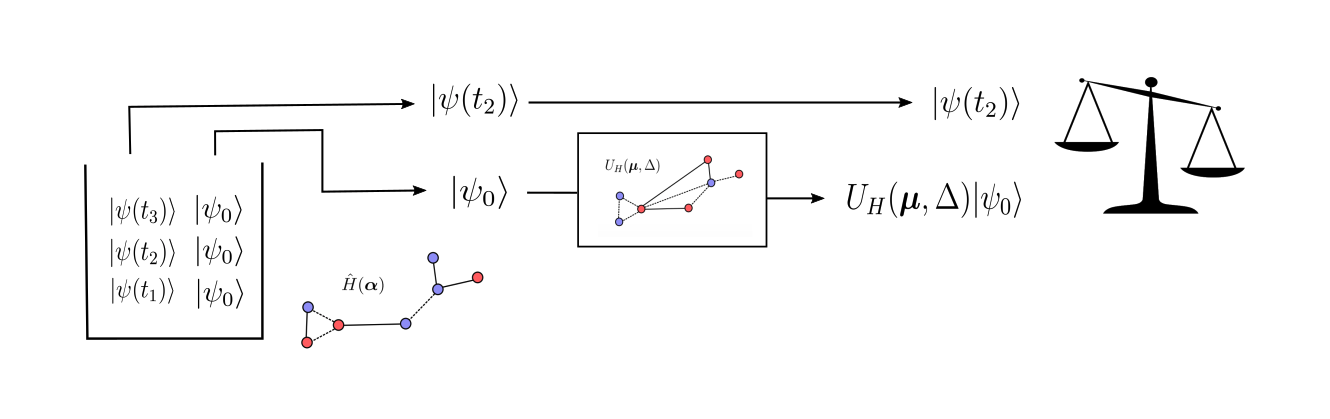
A visual representation of one execution of the QGRNN for one piece of quantum data.

Learning an Ising Model with the QGRNN

We now attempt to use the QGRNN to learn the parameters corresponding to an arbitrary transverse-field Ising model Hamiltonian.

Getting Started

We begin by importing the necessary dependencies:

import pennylane as qml
from matplotlib import pyplot as plt
from pennylane import numpy as np
import scipy
import networkx as nx
import copy

We also define some fixed values that are used throughout the simulation.

qubit_number = 4
qubits = range(qubit_number)

In this simulation, we don’t have quantum data readily available to pass into the QGRNN, so we have to generate it ourselves. To do this, we must have knowledge of the target interaction graph and the target Hamiltonian.

Let us use the following cyclic graph as the target interaction graph of the Ising Hamiltonian:

ising_graph = nx.cycle_graph(qubit_number)

print(f"Edges: {ising_graph.edges}")
nx.draw(ising_graph)

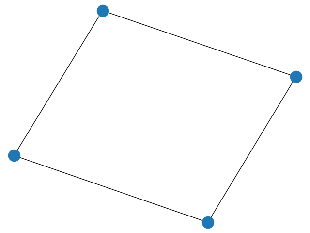
Out:

Edges: [(0, 1), (0, 3), (1, 2), (2, 3)]

We can then initialize the “unknown” target parameters that describe the target Hamiltonian, \(\boldsymbol\alpha \ = \ \{\alpha^{(1)}, \ \alpha^{(2)}\}\). Recall from the introduction that we have defined our parametrized Ising Hamiltonian to be of the form:

\[\hat{H}_{\text{Ising}}(\boldsymbol\theta) \ = \ \displaystyle\sum_{(i, j) \in E} \theta_{ij}^{(1)} Z_{i} Z_{j} \ + \ \displaystyle\sum_{i} \theta_{i}^{(2)} Z_{i} \ + \ \displaystyle\sum_{i} X_{i},\]

where \(E\) is the set of edges in the interaction graph, and \(X_i\) and \(Z_i\) are the Pauli-X and Pauli-Z on the \(i\)-th qubit.

For this tutorial, we choose the target parameters by sampling from a uniform probability distribution ranging from \(-2\) to \(2\), with two-decimal precision.

target_weights = [0.56, 1.24, 1.67, -0.79]
target_bias = [-1.44, -1.43, 1.18, -0.93]

In theory, these parameters can be any value we want, provided they are reasonably small enough that the QGRNN can reach them in a tractable number of optimization steps. In matrix_params, the first list represents the \(ZZ\) interaction parameters and the second list represents the single-qubit \(Z\) parameters.

Finally, we use this information to generate the matrix form of the Ising model Hamiltonian in the computational basis:

def create_hamiltonian_matrix(n_qubits, graph, weights, bias):

    full_matrix = np.zeros((2 ** n_qubits, 2 ** n_qubits))

    # Creates the interaction component of the Hamiltonian
    for i, edge in enumerate(graph.edges):
        interaction_term = 1
        for qubit in range(0, n_qubits):
            if qubit in edge:
                interaction_term = np.kron(interaction_term, qml.matrix(qml.PauliZ)(0))
            else:
                interaction_term = np.kron(interaction_term, np.identity(2))
        full_matrix += weights[i] * interaction_term

    # Creates the bias components of the matrix
    for i in range(0, n_qubits):
        z_term = x_term = 1
        for j in range(0, n_qubits):
            if j == i:
                z_term = np.kron(z_term, qml.matrix(qml.PauliZ)(0))
                x_term = np.kron(x_term, qml.matrix(qml.PauliX)(0))
            else:
                z_term = np.kron(z_term, np.identity(2))
                x_term = np.kron(x_term, np.identity(2))
        full_matrix += bias[i] * z_term + x_term

    return full_matrix


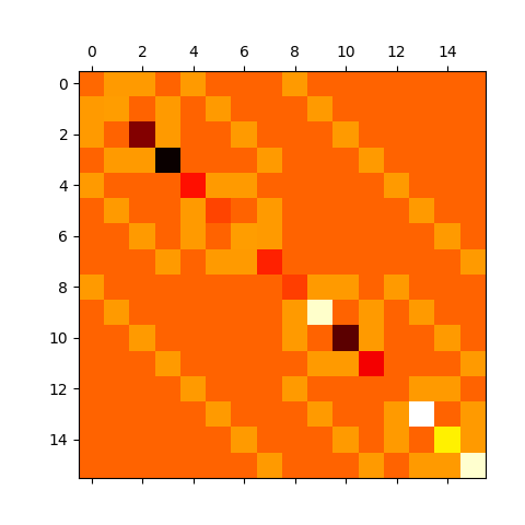
# Prints a visual representation of the Hamiltonian matrix
ham_matrix = create_hamiltonian_matrix(qubit_number, ising_graph, target_weights, target_bias)
plt.matshow(ham_matrix, cmap="hot")
plt.show()

Preparing Quantum Data

The collection of quantum data needed to run the QGRNN has two components: (i) copies of a low-energy state, and (ii) a collection of time-evolved states, each of which are simply the low-energy state evolved to different times. The following is a low-energy state of the target Hamiltonian:

low_energy_state = [
    (-0.054661080280306085 + 0.016713907320174026j),
    (0.12290003656489545 - 0.03758500591109822j),
    (0.3649337966440005 - 0.11158863596657455j),
    (-0.8205175732627094 + 0.25093231967092877j),
    (0.010369790825776609 - 0.0031706387262686003j),
    (-0.02331544978544721 + 0.007129899300113728j),
    (-0.06923183949694546 + 0.0211684344103713j),
    (0.15566094863283836 - 0.04760201916285508j),
    (0.014520590919500158 - 0.004441887836078486j),
    (-0.032648113364535575 + 0.009988590222879195j),
    (-0.09694382811137187 + 0.02965579457620536j),
    (0.21796861485652747 - 0.06668776658411019j),
    (-0.0027547112135013247 + 0.0008426289322652901j),
    (0.006193695872468649 - 0.0018948418969390599j),
    (0.018391279795405405 - 0.005625722994009138j),
    (-0.041350974715649635 + 0.012650711602265649j),
]

This state can be obtained by using a decoupled version of the Variational Quantum Eigensolver algorithm (VQE). Essentially, we choose a VQE ansatz such that the circuit cannot learn the exact ground state, but it can get fairly close. Another way to arrive at the same result is to perform VQE with a reasonable ansatz, but to terminate the algorithm before it converges to the ground state. If we used the exact ground state \(|\psi_0\rangle\), the time-dependence would be trivial and the data would not provide enough information about the Hamiltonian parameters.

We can verify that this is a low-energy state by numerically finding the lowest eigenvalue of the Hamiltonian and comparing it to the energy expectation of this low-energy state:

res = np.vdot(low_energy_state, (ham_matrix @ low_energy_state))
energy_exp = np.real_if_close(res)
print(f"Energy Expectation: {energy_exp}")


ground_state_energy = np.real_if_close(min(np.linalg.eig(ham_matrix)[0]))
print(f"Ground State Energy: {ground_state_energy}")

Out:

Energy Expectation: -7.244508985189116
Ground State Energy: -7.330689661291261

We have in fact found a low-energy, non-ground state, as the energy expectation is slightly greater than the energy of the true ground state. This, however, is only half of the information we need. We also require a collection of time-evolved, low-energy states. Evolving the low-energy state forward in time is fairly straightforward: all we have to do is multiply the initial state by a time-evolution unitary. This operation can be defined as a custom gate in PennyLane:

def state_evolve(hamiltonian, qubits, time):

    U = scipy.linalg.expm(-1j * hamiltonian * time)
    qml.QubitUnitary(U, wires=qubits)

We don’t actually generate time-evolved quantum data quite yet, but we now have all the pieces required for its preparation.

Learning the Hamiltonian

With the quantum data defined, we are able to construct the QGRNN and learn the target Hamiltonian. Each of the exponentiated Hamiltonians in the QGRNN ansatz, \(\hat{H}^{j}_{\text{Ising}}(\boldsymbol\mu)\), are the \(ZZ\), \(Z\), and \(X\) terms from the Ising Hamiltonian. This gives:

def qgrnn_layer(weights, bias, qubits, graph, trotter_step):

    # Applies a layer of RZZ gates (based on a graph)
    for i, edge in enumerate(graph.edges):
        qml.MultiRZ(2 * weights[i] * trotter_step, wires=(edge[0], edge[1]))

    # Applies a layer of RZ gates
    for i, qubit in enumerate(qubits):
        qml.RZ(2 * bias[i] * trotter_step, wires=qubit)

    # Applies a layer of RX gates
    for qubit in qubits:
        qml.RX(2 * trotter_step, wires=qubit)

As was mentioned in the first section, the QGRNN has two registers. In one register, some piece of quantum data \(|\psi(t)\rangle\) is prepared and in the other we have \(U_{H}(\boldsymbol\mu, \ \Delta) |\psi_0\rangle\). We need a way to measure the similarity between these states. This can be done by using the fidelity, which is simply the modulus squared of the inner product between the states, \(| \langle \psi(t) | U_{H}(\Delta, \ \boldsymbol\mu) |\psi_0\rangle |^2\). To calculate this value, we use a SWAP test between the registers:

def swap_test(control, register1, register2):

    qml.Hadamard(wires=control)
    for reg1_qubit, reg2_qubit in zip(register1, register2):
        qml.CSWAP(wires=(control, reg1_qubit, reg2_qubit))
    qml.Hadamard(wires=control)

After performing this procedure, the value returned from a measurement of the circuit is \(\langle Z \rangle\), with respect to the control qubit. The probability of measuring the \(|0\rangle\) state in this control qubit is related to both the fidelity between registers and \(\langle Z \rangle\). Thus, with a bit of algebra, we find that \(\langle Z \rangle\) is equal to the fidelity.

Before creating the full QGRNN and the cost function, we define a few more fixed values. Among these is a “guessed” interaction graph, which we set to be a complete graph. This choice is motivated by the fact that any target interaction graph will be a subgraph of this initial guess. Part of the idea behind the QGRNN is that we don’t know the interaction graph, and it has to be learned. In this case, the graph is learned automatically as the target parameters are optimized. The \(\boldsymbol\mu\) parameters that correspond to edges that don’t exist in the target graph will simply approach \(0\).

# Defines some fixed values

reg1 = tuple(range(qubit_number))  # First qubit register
reg2 = tuple(range(qubit_number, 2 * qubit_number))  # Second qubit register

control = 2 * qubit_number  # Index of control qubit
trotter_step = 0.01  # Trotter step size

# Defines the interaction graph for the new qubit system

new_ising_graph = nx.complete_graph(reg2)

print(f"Edges: {new_ising_graph.edges}")
nx.draw(new_ising_graph)

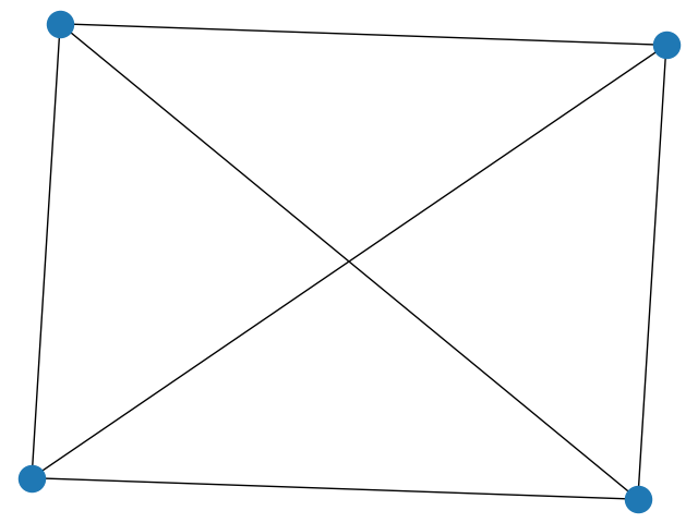
Out:

Edges: [(4, 5), (4, 6), (4, 7), (5, 6), (5, 7), (6, 7)]

With this done, we implement the QGRNN circuit for some given time value:

def qgrnn(weights, bias, time=None):

    # Prepares the low energy state in the two registers
    qml.QubitStateVector(np.kron(low_energy_state, low_energy_state), wires=reg1 + reg2)

    # Evolves the first qubit register with the time-evolution circuit to
    # prepare a piece of quantum data
    state_evolve(ham_matrix, reg1, time)

    # Applies the QGRNN layers to the second qubit register
    depth = time / trotter_step  # P = t/Delta
    for _ in range(0, int(depth)):
        qgrnn_layer(weights, bias, reg2, new_ising_graph, trotter_step)

    # Applies the SWAP test between the registers
    swap_test(control, reg1, reg2)

    # Returns the results of the SWAP test
    return qml.expval(qml.PauliZ(control))

We have the full QGRNN circuit, but we still need to define a cost function. We know that \(| \langle \psi(t) | U_{H}(\boldsymbol\mu, \ \Delta) |\psi_0\rangle |^2\) approaches \(1\) as the states become more similar and approaches \(0\) as the states become orthogonal. Thus, we choose to minimize the quantity \(-| \langle \psi(t) | U_{H}(\boldsymbol\mu, \ \Delta) |\psi_0\rangle |^2\). Since we are interested in calculating this value for many different pieces of quantum data, the final cost function is the average negative fidelity* between registers:

\[\mathcal{L}(\boldsymbol\mu, \ \Delta) \ = \ - \frac{1}{N} \displaystyle\sum_{i \ = \ 1}^{N} | \langle \psi(t_i) | \ U_{H}(\boldsymbol\mu, \ \Delta) \ |\psi_0\rangle |^2,\]

where we use \(N\) pieces of quantum data.

Before creating the cost function, we must define a few more fixed variables:

N = 15  # The number of pieces of quantum data that are used for each step
max_time = 0.1  # The maximum value of time that can be used for quantum data

We then define the negative fidelity cost function:

rng = np.random.default_rng(seed=42)

def cost_function(weight_params, bias_params):

    # Randomly samples times at which the QGRNN runs
    times_sampled = rng.random(size=N) * max_time

    # Cycles through each of the sampled times and calculates the cost
    total_cost = 0
    for dt in times_sampled:
        result = qgrnn_qnode(weight_params, bias_params, time=dt)
        total_cost += -1 * result

    return total_cost / N

Next we set up for optimization.

# Defines the new device
qgrnn_dev = qml.device("default.qubit", wires=2 * qubit_number + 1)

# Defines the new QNode
qgrnn_qnode = qml.QNode(qgrnn, qgrnn_dev, interface="autograd")

steps = 300

optimizer = qml.AdamOptimizer(stepsize=0.5)

weights = rng.random(size=len(new_ising_graph.edges), requires_grad=True) - 0.5
bias = rng.random(size=qubit_number, requires_grad=True) - 0.5

initial_weights = copy.copy(weights)
initial_bias = copy.copy(bias)

All that remains is executing the optimization loop.

for i in range(0, steps):
    (weights, bias), cost = optimizer.step_and_cost(cost_function, weights, bias)

    # Prints the value of the cost function
    if i % 5 == 0:
        print(f"Cost at Step {i}: {cost}")
        print(f"Weights at Step {i}: {weights}")
        print(f"Bias at Step {i}: {bias}")
        print("---------------------------------------------")

Out:

Cost at Step 0: -0.9803638573791951
Weights at Step 0: [-0.22603613  0.43887001  0.85859236  0.69735898  0.09417125 -0.02437147]
Bias at Step 0: [-0.23884748 -0.21392016  0.12809368  0.45037793]
---------------------------------------------
Cost at Step 5: -0.9974589524428065
Weights at Step 5: [-0.75106068  1.078707    0.83766935  1.9741555   0.04982793 -0.06747815]
Bias at Step 5: [-0.50836435 -1.32708118  1.57468372  0.11442806]
---------------------------------------------
Cost at Step 10: -0.9971878268304836
Weights at Step 10: [ 0.01577799  0.48771566  0.68379977  1.75747002 -0.21948418 -0.00484698]
Bias at Step 10: [ 0.22007905 -0.90282076  1.58989008 -0.1051542 ]
---------------------------------------------
Cost at Step 15: -0.9981871533122783
Weights at Step 15: [-0.06744249  0.65720464  1.31471457  1.47430241  0.05813038 -0.41315658]
Bias at Step 15: [-0.29045223 -0.67045595  1.19395446  0.24677711]
---------------------------------------------
Cost at Step 20: -0.9995130692146906
Weights at Step 20: [-0.16225009  0.66208813  1.17758061  1.48254064 -0.35468207 -0.01648733]
Bias at Step 20: [-0.56832881 -0.87721581  0.86890622 -0.27734217]
---------------------------------------------
Cost at Step 25: -0.9998181560069601
Weights at Step 25: [ 0.030689    0.40363412  1.32430282  1.80692972 -0.14761078 -0.27452275]
Bias at Step 25: [-0.33695681 -1.28646051  1.00509121 -0.19672993]
---------------------------------------------
Cost at Step 30: -0.9997713453918171
Weights at Step 30: [ 0.22014178  0.38063046  1.34934589  1.82854127 -0.201276   -0.35610913]
Bias at Step 30: [-0.40515586 -1.19466624  1.13933672 -0.31753371]
---------------------------------------------
Cost at Step 35: -0.9997858632135197
Weights at Step 35: [ 0.22310889  0.50896099  1.36029033  1.73588161 -0.30076632 -0.35201799]
Bias at Step 35: [-0.73605504 -1.06150682  1.07911402 -0.49331792]
---------------------------------------------
Cost at Step 40: -0.9998587245201078
Weights at Step 40: [ 0.32580831  0.34293483  1.38813471  1.76261455 -0.16880133 -0.49831078]
Bias at Step 40: [-0.74534508 -1.20379495  0.91916721 -0.49099848]
---------------------------------------------
Cost at Step 45: -0.9998796449154754
Weights at Step 45: [ 0.37151473  0.26329833  1.29149206  1.84754531 -0.16287055 -0.51793342]
Bias at Step 45: [-0.81082195 -1.35860008  0.88788716 -0.63818331]
---------------------------------------------
Cost at Step 50: -0.9999381279674843
Weights at Step 50: [ 0.36839385  0.36200243  1.3398256   1.82138962 -0.10863003 -0.63499473]
Bias at Step 50: [-1.04909977 -1.27581779  0.93902928 -0.67286639]
---------------------------------------------
Cost at Step 55: -0.999925288139168
Weights at Step 55: [ 0.52717503  0.22669791  1.27477846  1.75733597 -0.1195999  -0.66147384]
Bias at Step 55: [-1.02458911 -1.19668936  0.89787258 -0.76851797]
---------------------------------------------
Cost at Step 60: -0.9999298586216679
Weights at Step 60: [ 0.46426344  0.2377941   1.30579533  1.86309089 -0.05164041 -0.72495523]
Bias at Step 60: [-1.15189323 -1.3565901   0.92299357 -0.81716179]
---------------------------------------------
Cost at Step 65: -0.9999633163685169
Weights at Step 65: [ 0.54814165  0.15321249  1.29421602  1.79468038 -0.06551864 -0.73442872]
Bias at Step 65: [-1.18093812 -1.2850757   0.8715214  -0.89498456]
---------------------------------------------
Cost at Step 70: -0.9999692974112414
Weights at Step 70: [ 0.54968362  0.15363051  1.32636004  1.81799545 -0.03795287 -0.78176424]
Bias at Step 70: [-1.26004878 -1.29186174  0.93275685 -0.93151559]
---------------------------------------------
Cost at Step 75: -0.9999839418036033
Weights at Step 75: [ 0.56926778  0.09899053  1.32784104  1.83800055 -0.02258999 -0.80100631]
Bias at Step 75: [-1.27844754 -1.32707392  0.95121289 -0.97776518]
---------------------------------------------
Cost at Step 80: -0.9999900754964208
Weights at Step 80: [ 0.58436296  0.06469565  1.33177097  1.80638755 -0.0264562  -0.80504093]
Bias at Step 80: [-1.32003524 -1.30314422  0.93367031 -1.02093595]
---------------------------------------------
Cost at Step 85: -0.9999892005586446
Weights at Step 85: [ 5.76118484e-01  5.92975577e-02  1.35458994e+00  1.82562544e+00
 -6.90843714e-04 -8.37859294e-01]
Bias at Step 85: [-1.35783384 -1.32173749  0.97374052 -1.02956436]
---------------------------------------------
Cost at Step 90: -0.9999860418671456
Weights at Step 90: [ 0.60406684  0.01793718  1.33218637  1.81633306 -0.0189833  -0.82575128]
Bias at Step 90: [-1.35074923 -1.31381294  0.98189172 -1.07270478]
---------------------------------------------
Cost at Step 95: -0.9999837519650716
Weights at Step 95: [ 0.58241323  0.02570679  1.35041725  1.81039596  0.00900262 -0.85399323]
Bias at Step 95: [-1.39511753 -1.32055157  0.98642234 -1.06137202]
---------------------------------------------
Cost at Step 100: -0.9999862374755413
Weights at Step 100: [ 0.59133649  0.00671959  1.33149619  1.80654252  0.00739735 -0.85271751]
Bias at Step 100: [-1.3928395  -1.32434117  0.99986843 -1.0746036 ]
---------------------------------------------
Cost at Step 105: -0.9999860417314536
Weights at Step 105: [ 5.98294601e-01 -1.63872117e-03  1.32435903e+00  1.79606830e+00
 -1.50600209e-03 -8.46854780e-01]
Bias at Step 105: [-1.39810406 -1.31716394  1.00632966 -1.08694727]
---------------------------------------------
Cost at Step 110: -0.9999889448376583
Weights at Step 110: [ 0.58790075  0.00252021  1.34070893  1.79969067  0.01353978 -0.86073241]
Bias at Step 110: [-1.41237809 -1.33237829  1.01344356 -1.07306401]
---------------------------------------------
Cost at Step 115: -0.9999907527375081
Weights at Step 115: [ 0.59511523 -0.00485992  1.33269226  1.79443191  0.00548165 -0.85246429]
Bias at Step 115: [-1.40713813 -1.33369881  1.02023634 -1.07811166]
---------------------------------------------
Cost at Step 120: -0.9999894991115524
Weights at Step 120: [ 5.96065192e-01 -3.92737036e-03  1.33288381e+00  1.78858855e+00
  1.75644333e-03 -8.48477853e-01]
Bias at Step 120: [-1.40998319 -1.33422301  1.02362295 -1.07680692]
---------------------------------------------
Cost at Step 125: -0.9999921833903894
Weights at Step 125: [ 5.91985767e-01 -1.57241251e-03  1.33882177e+00  1.79191152e+00
  8.89983556e-03 -8.53306759e-01]
Bias at Step 125: [-1.41164517 -1.34685868  1.0288417  -1.06603474]
---------------------------------------------
Cost at Step 130: -0.9999895629847527
Weights at Step 130: [ 5.93396935e-01 -6.09903975e-04  1.32769014e+00  1.78340627e+00
  3.20989912e-03 -8.45936030e-01]
Bias at Step 130: [-1.41153989 -1.34372306  1.0306921  -1.06641934]
---------------------------------------------
Cost at Step 135: -0.9999893671898585
Weights at Step 135: [ 5.93933082e-01 -1.84879055e-04  1.32433785e+00  1.77929886e+00
  4.38714188e-03 -8.45503125e-01]
Bias at Step 135: [-1.4098866  -1.34497204  1.03415862 -1.06007092]
---------------------------------------------
Cost at Step 140: -0.9999909995915355
Weights at Step 140: [ 0.5908483   0.00239647  1.33016899  1.78168215  0.00438378 -0.84478361]
Bias at Step 140: [-1.41145547 -1.35249113  1.0371159  -1.05630093]
---------------------------------------------
Cost at Step 145: -0.9999882781659966
Weights at Step 145: [ 5.95379262e-01 -3.85481762e-04  1.33209614e+00  1.77901613e+00
 -1.07423798e-03 -8.40357066e-01]
Bias at Step 145: [-1.40745547 -1.35117282  1.03764696 -1.05779208]
---------------------------------------------
Cost at Step 150: -0.9999882605157393
Weights at Step 150: [ 0.59753863 -0.00178702  1.33577445  1.78058366 -0.00414765 -0.83825161]
Bias at Step 150: [-1.40514789 -1.35375725  1.03826782 -1.05953418]
---------------------------------------------
Cost at Step 155: -0.9999873092858359
Weights at Step 155: [ 5.96677467e-01  6.17989620e-04  1.34466485e+00  1.78402267e+00
 -2.65741532e-03 -8.41450495e-01]
Bias at Step 155: [-1.40789298 -1.356471    1.0376034  -1.05877886]
---------------------------------------------
Cost at Step 160: -0.9999872637771781
Weights at Step 160: [ 0.60194839 -0.00191478  1.35123357  1.7884694  -0.00603744 -0.84142449]
Bias at Step 160: [-1.40510396 -1.35668892  1.03451132 -1.06543631]
---------------------------------------------
Cost at Step 165: -0.9999874624869814
Weights at Step 165: [ 0.6030402  -0.00193504  1.34611742  1.78890714 -0.00577061 -0.84238872]
Bias at Step 165: [-1.40613555 -1.35445251  1.02812253 -1.07090041]
---------------------------------------------
Cost at Step 170: -0.9999886747321731
Weights at Step 170: [ 0.5975333   0.00282116  1.32780927  1.78277225  0.00466827 -0.84919749]
Bias at Step 170: [-1.41126245 -1.34857858  1.02684163 -1.0645541 ]
---------------------------------------------
Cost at Step 175: -0.9999875562507266
Weights at Step 175: [ 0.59389571  0.00440434  1.32168971  1.78088367  0.00772899 -0.85019789]
Bias at Step 175: [-1.41279703 -1.34685714  1.02847119 -1.06186318]
---------------------------------------------
Cost at Step 180: -0.9999914836764869
Weights at Step 180: [ 5.95476507e-01  1.04646713e-03  1.33253375e+00  1.78379408e+00
  1.79045580e-03 -8.45539923e-01]
Bias at Step 180: [-1.40924345 -1.34843997  1.03054894 -1.06465758]
---------------------------------------------
Cost at Step 185: -0.9999877384049646
Weights at Step 185: [ 0.60021817 -0.00344807  1.34837992  1.78919267 -0.00485391 -0.84211998]
Bias at Step 185: [-1.40406354 -1.35059434  1.03159602 -1.06906187]
---------------------------------------------
Cost at Step 190: -0.999994381128065
Weights at Step 190: [ 0.60332647 -0.00502377  1.35580211  1.7937833  -0.00870162 -0.84089377]
Bias at Step 190: [-1.40248031 -1.35189812  1.02840358 -1.07489377]
---------------------------------------------
Cost at Step 195: -0.9999899532834544
Weights at Step 195: [ 6.01661213e-01 -1.40258189e-03  1.34845381e+00  1.79177947e+00
 -2.19330435e-03 -8.46882171e-01]
Bias at Step 195: [-1.40624231 -1.34827409  1.02488298 -1.07228167]
---------------------------------------------
Cost at Step 200: -0.9999880990041669
Weights at Step 200: [ 0.59781588  0.00262681  1.33622645  1.7903236   0.00491206 -0.85187394]
Bias at Step 200: [-1.41001483 -1.3468901   1.02276916 -1.06950677]
---------------------------------------------
Cost at Step 205: -0.9999882388738703
Weights at Step 205: [ 0.59525242  0.00459556  1.33045933  1.78843797  0.00647584 -0.85208423]
Bias at Step 205: [-1.41193406 -1.34513748  1.02230177 -1.06854427]
---------------------------------------------
Cost at Step 210: -0.9999848077040225
Weights at Step 210: [ 0.59407847  0.00331191  1.3261464   1.78462336  0.00583158 -0.84928496]
Bias at Step 210: [-1.40995186 -1.34363827  1.02517197 -1.06554306]
---------------------------------------------
Cost at Step 215: -0.9999886167575471
Weights at Step 215: [ 5.93598280e-01  1.27457027e-03  1.32894414e+00  1.78302258e+00
  3.44879382e-03 -8.45638843e-01]
Bias at Step 215: [-1.40701621 -1.34498189  1.03023459 -1.06215846]
---------------------------------------------
Cost at Step 220: -0.9999875727826226
Weights at Step 220: [ 5.94793970e-01 -8.57403941e-04  1.33609793e+00  1.78453102e+00
 -2.17937735e-03 -8.40640138e-01]
Bias at Step 220: [-1.40459538 -1.34840612  1.03328985 -1.06323676]
---------------------------------------------
Cost at Step 225: -0.9999895237582359
Weights at Step 225: [ 0.59740767 -0.00202435  1.33963888  1.78462403 -0.00566848 -0.83842794]
Bias at Step 225: [-1.40352872 -1.34909283  1.03367034 -1.0646202 ]
---------------------------------------------
Cost at Step 230: -0.9999922217151871
Weights at Step 230: [ 0.59830589 -0.00184753  1.33406652  1.78177535 -0.00330205 -0.84015047]
Bias at Step 230: [-1.40427031 -1.34839966  1.03168677 -1.06292291]
---------------------------------------------
Cost at Step 235: -0.9999912692867956
Weights at Step 235: [ 5.95836686e-01  8.57240159e-04  1.32786532e+00  1.78035155e+00
  2.56153005e-03 -8.44403818e-01]
Bias at Step 235: [-1.40725255 -1.34955664  1.03260437 -1.05840103]
---------------------------------------------
Cost at Step 240: -0.9999899357699936
Weights at Step 240: [ 0.59351612  0.00209534  1.32485259  1.77824259  0.00444528 -0.8447466 ]
Bias at Step 240: [-1.40903945 -1.35042747  1.03478287 -1.05550792]
---------------------------------------------
Cost at Step 245: -0.9999889869569236
Weights at Step 245: [ 5.95395532e-01  1.23721713e-03  1.33593185e+00  1.78146341e+00
 -1.83303336e-03 -8.40987115e-01]
Bias at Step 245: [-1.40856761 -1.35225776  1.03748333 -1.05978839]
---------------------------------------------
Cost at Step 250: -0.9999881293170535
Weights at Step 250: [ 5.95495047e-01 -2.18886873e-04  1.33760142e+00  1.78252108e+00
 -1.04388862e-03 -8.41650674e-01]
Bias at Step 250: [-1.40788422 -1.35473503  1.03617744 -1.05980154]
---------------------------------------------
Cost at Step 255: -0.999989261380938
Weights at Step 255: [ 5.95095996e-01  1.05345945e-03  1.33120954e+00  1.78110699e+00
  9.09621038e-04 -8.43176791e-01]
Bias at Step 255: [-1.40881827 -1.35271576  1.03732158 -1.05936317]
---------------------------------------------
Cost at Step 260: -0.9999911696516867
Weights at Step 260: [ 0.59215329  0.00249312  1.32162048  1.77469111  0.00411753 -0.84385295]
Bias at Step 260: [-1.41164782 -1.34921326  1.03505213 -1.05565234]
---------------------------------------------
Cost at Step 265: -0.9999897602169328
Weights at Step 265: [ 5.94219509e-01  1.15801805e-03  1.32981272e+00  1.77875998e+00
  2.00797690e-03 -8.43338459e-01]
Bias at Step 265: [-1.40879199 -1.35161558  1.04052305 -1.05548315]
---------------------------------------------
Cost at Step 270: -0.9999877865048095
Weights at Step 270: [ 0.5967199  -0.00228699  1.34015592  1.78207987 -0.00207472 -0.8407702 ]
Bias at Step 270: [-1.40654726 -1.35550984  1.03685756 -1.05892969]
---------------------------------------------
Cost at Step 275: -0.9999913148930926
Weights at Step 275: [ 5.95115179e-01  6.67458889e-04  1.33088691e+00  1.77908492e+00
  2.17950090e-03 -8.43784743e-01]
Bias at Step 275: [-1.40907272 -1.35232601  1.03787329 -1.05577319]
---------------------------------------------
Cost at Step 280: -0.9999912773774007
Weights at Step 280: [ 5.94534323e-01  1.49825127e-03  1.33221200e+00  1.78129607e+00
  1.80930063e-03 -8.43864609e-01]
Bias at Step 280: [-1.41032893 -1.35393432  1.03609549 -1.0579392 ]
---------------------------------------------
Cost at Step 285: -0.9999871922879695
Weights at Step 285: [ 5.96437497e-01  3.12450031e-04  1.33601315e+00  1.78353853e+00
 -7.60576311e-04 -8.42698914e-01]
Bias at Step 285: [-1.40896079 -1.3539148   1.03483345 -1.06189856]
---------------------------------------------
Cost at Step 290: -0.9999918144420561
Weights at Step 290: [ 0.5928268   0.00288728  1.32568915  1.77748739  0.00484885 -0.84553166]
Bias at Step 290: [-1.41115856 -1.34928842  1.03616776 -1.0560555 ]
---------------------------------------------
Cost at Step 295: -0.9999908668757269
Weights at Step 295: [ 5.95067478e-01  6.59873701e-06  1.33530656e+00  1.78268285e+00
 -6.83963342e-04 -8.41953097e-01]
Bias at Step 295: [-1.40781716 -1.35320774  1.03673384 -1.06074438]
---------------------------------------------

With the learned parameters, we construct a visual representation of the Hamiltonian to which they correspond and compare it to the target Hamiltonian, and the initial guessed Hamiltonian:

new_ham_matrix = create_hamiltonian_matrix(
    qubit_number, nx.complete_graph(qubit_number), weights, bias
)

init_ham = create_hamiltonian_matrix(
    qubit_number, nx.complete_graph(qubit_number), initial_weights, initial_bias
)

fig, axes = plt.subplots(nrows=1, ncols=3, figsize=(6, 6))

axes[0].matshow(ham_matrix, vmin=-7, vmax=7, cmap="hot")
axes[0].set_title("Target", y=1.13)

axes[1].matshow(init_ham, vmin=-7, vmax=7, cmap="hot")
axes[1].set_title("Initial", y=1.13)

axes[2].matshow(new_ham_matrix, vmin=-7, vmax=7, cmap="hot")
axes[2].set_title("Learned", y=1.13)

plt.subplots_adjust(wspace=0.3, hspace=0.3)
plt.show()

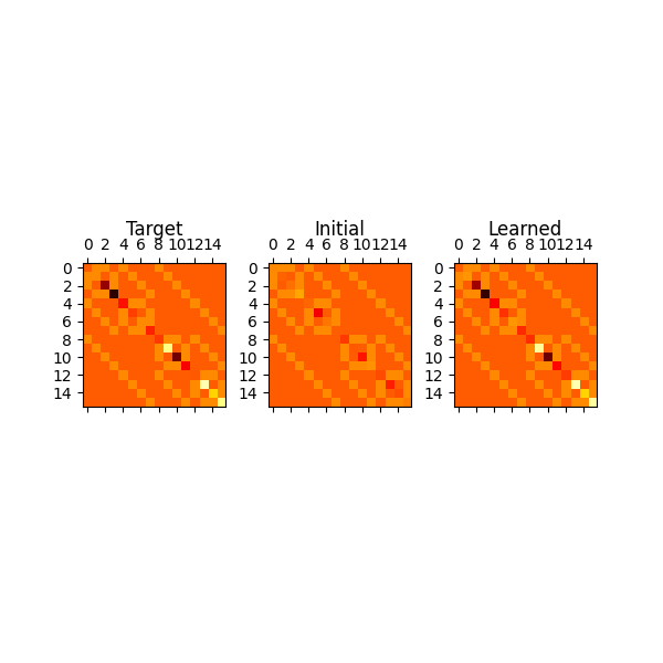
These images look very similar, indicating that the QGRNN has done a good job learning the target Hamiltonian.

We can also look at the exact values of the target and learned parameters. Recall how the target interaction graph has \(4\) edges while the complete graph has \(6\). Thus, as the QGRNN converges to the optimal solution, the weights corresponding to edges \((1, 3)\) and \((2, 0)\) in the complete graph should go to \(0\), as this indicates that they have no effect, and effectively do not exist in the learned Hamiltonian.

# We first pick out the weights of edges (1, 3) and (2, 0)
# and then remove them from the list of target parameters

weights_noedge = []
weights_edge = []
for ii, edge in enumerate(new_ising_graph.edges):
    if (edge[0] - qubit_number, edge[1] - qubit_number) in ising_graph.edges:
        weights_edge.append(weights[ii])
    else:
        weights_noedge.append(weights[ii])

Then, we print all of the weights:

print("Target parameters     Learned parameters")
print("Weights")
print("-" * 41)
for ii_target, ii_learned in zip(target_weights, weights_edge):
    print(f"{ii_target : <20}|{ii_learned : >20}")

print("\nBias")
print("-"*41)
for ii_target, ii_learned in zip(target_bias, bias):
    print(f"{ii_target : <20}|{ii_learned : >20}")

print(f"\nNon-Existing Edge Parameters: {[val.unwrap() for val in weights_noedge]}")

Out:

Target parameters     Learned parameters
Weights
-----------------------------------------
0.56                |  0.5988034096092802
1.24                |  1.3483865512005315
1.67                |  1.7862070648455897
-0.79               | -0.8425475506159242

Bias
-----------------------------------------
-1.44               | -1.4067983643944135
-1.43               | -1.3529638627173872
1.18                |  1.0349129419830776
-0.93               | -1.0635874966599637

Non-Existing Edge Parameters: [-0.0012651471928184215, -0.003653447242320976]

The weights of edges \((1, 3)\) and \((2, 0)\) are very close to \(0\), indicating we have learned the cycle graph from the complete graph. In addition, the remaining learned weights are fairly close to those of the target Hamiltonian. Thus, the QGRNN is functioning properly, and has learned the target Ising Hamiltonian to a high degree of accuracy!

References

1. Verdon, G., McCourt, T., Luzhnica, E., Singh, V., Leichenauer, S., & Hidary, J. (2019). Quantum Graph Neural Networks. arXiv preprint arXiv:1909.12264.

About the author

Jack Ceroni

Jack is currently a second-year undergraduate student at the University of Toronto, pursuing a degree in pure mathematics. Broadly, his interests are related to simulating quantum systems with quantum computers, mathematical abstraction, and philosophy.

demos/tutorial_qgrnn

 

Download Python script

 

Download Notebook

 

View on GitHub