A brief overview of VQE

Author: Alain Delgado — Posted: 08 February 2020. Last updated: 25 June 2022.

The Variational Quantum Eigensolver (VQE) is a flagship algorithm for quantum chemistry using near-term quantum computers 1. It is an application of the Ritz variational principle, where a quantum computer is trained to prepare the ground state of a given molecule.

The inputs to the VQE algorithm are a molecular Hamiltonian and a parametrized circuit preparing the quantum state of the molecule. Within VQE, the cost function is defined as the expectation value of the Hamiltonian computed in the trial state. The ground state of the target Hamiltonian is obtained by performing an iterative minimization of the cost function. The optimization is carried out by a classical optimizer which leverages a quantum computer to evaluate the cost function and calculate its gradient at each optimization step.

In this tutorial you will learn how to implement the VQE algorithm in a few lines of code. As an illustrative example, we use it to find the ground state of the hydrogen molecule, \(\mathrm{H}_2\). First, we build the molecular Hamiltonian using a minimal basis set approximation. Next, we design the quantum circuit preparing the trial state of the molecule, and the cost function to evaluate the expectation value of the Hamiltonian. Finally, we select a classical optimizer, initialize the circuit parameters, and run the VQE algorithm using a PennyLane simulator.

Let’s get started!

Building the electronic Hamiltonian

The first step is to specify the molecule we want to simulate. This is done by providing a list with the symbols of the constituent atoms and a one-dimensional array with the corresponding nuclear coordinates in atomic units.

from pennylane import numpy as np

symbols = ["H", "H"]
coordinates = np.array([0.0, 0.0, -0.6614, 0.0, 0.0, 0.6614])

The molecular structure can also be imported from an external file using the read_structure() function.

Now, we can build the electronic Hamiltonian of the hydrogen molecule using the molecular_hamiltonian() function.

import pennylane as qml

H, qubits = qml.qchem.molecular_hamiltonian(symbols, coordinates)
print("Number of qubits = ", qubits)
print("The Hamiltonian is ", H)

Out:

Number of qubits =  4
The Hamiltonian is    (-0.2427450126094144) [Z2]
+ (-0.2427450126094144) [Z3]
+ (-0.042072551947439224) [I0]
+ (0.1777135822909176) [Z0]
+ (0.1777135822909176) [Z1]
+ (0.12293330449299361) [Z0 Z2]
+ (0.12293330449299361) [Z1 Z3]
+ (0.16768338855601356) [Z0 Z3]
+ (0.16768338855601356) [Z1 Z2]
+ (0.17059759276836803) [Z0 Z1]
+ (0.1762766139418181) [Z2 Z3]
+ (-0.044750084063019925) [Y0 Y1 X2 X3]
+ (-0.044750084063019925) [X0 X1 Y2 Y3]
+ (0.044750084063019925) [Y0 X1 X2 Y3]
+ (0.044750084063019925) [X0 Y1 Y2 X3]

The outputs of the function are the Hamiltonian, represented as a linear combination of Pauli operators, and the number of qubits required for the quantum simulations. For this example, we use a minimal basis set to represent the molecular orbitals. In this approximation, we have four spin orbitals, which defines the number of qubits. Furthermore, we use the Jordan-Wigner transformation 2 to perform the fermionic-to-qubit mapping of the Hamiltonian.

For a more comprehensive discussion on how to build the Hamiltonian of more complicated molecules, see the tutorial Building molecular Hamiltonians.

Implementing the VQE algorithm

From here on, we can use PennyLane as usual, employing its entire stack of algorithms and optimizers. We begin by defining the device, in this case PennyLane’s standard qubit simulator:

dev = qml.device("default.qubit", wires=qubits)

Next, we need to define the quantum circuit that prepares the trial state of the molecule. We want to prepare states of the form,

\[\vert \Psi(\theta) \rangle = \cos(\theta/2)~|1100\rangle -\sin(\theta/2)~|0011\rangle,\]

where \(\theta\) is the variational parameter to be optimized in order to find the best approximation to the true ground state. In the Jordan-Wigner 2 encoding, the first term \(|1100\rangle\) represents the Hartree-Fock (HF) state where the two electrons in the molecule occupy the lowest-energy orbitals. The second term \(|0011\rangle\) encodes a double excitation of the HF state where the two particles are excited from qubits 0, 1 to 2, 3.

The quantum circuit to prepare the trial state \(\vert \Psi(\theta) \rangle\) is schematically illustrated in the figure below.

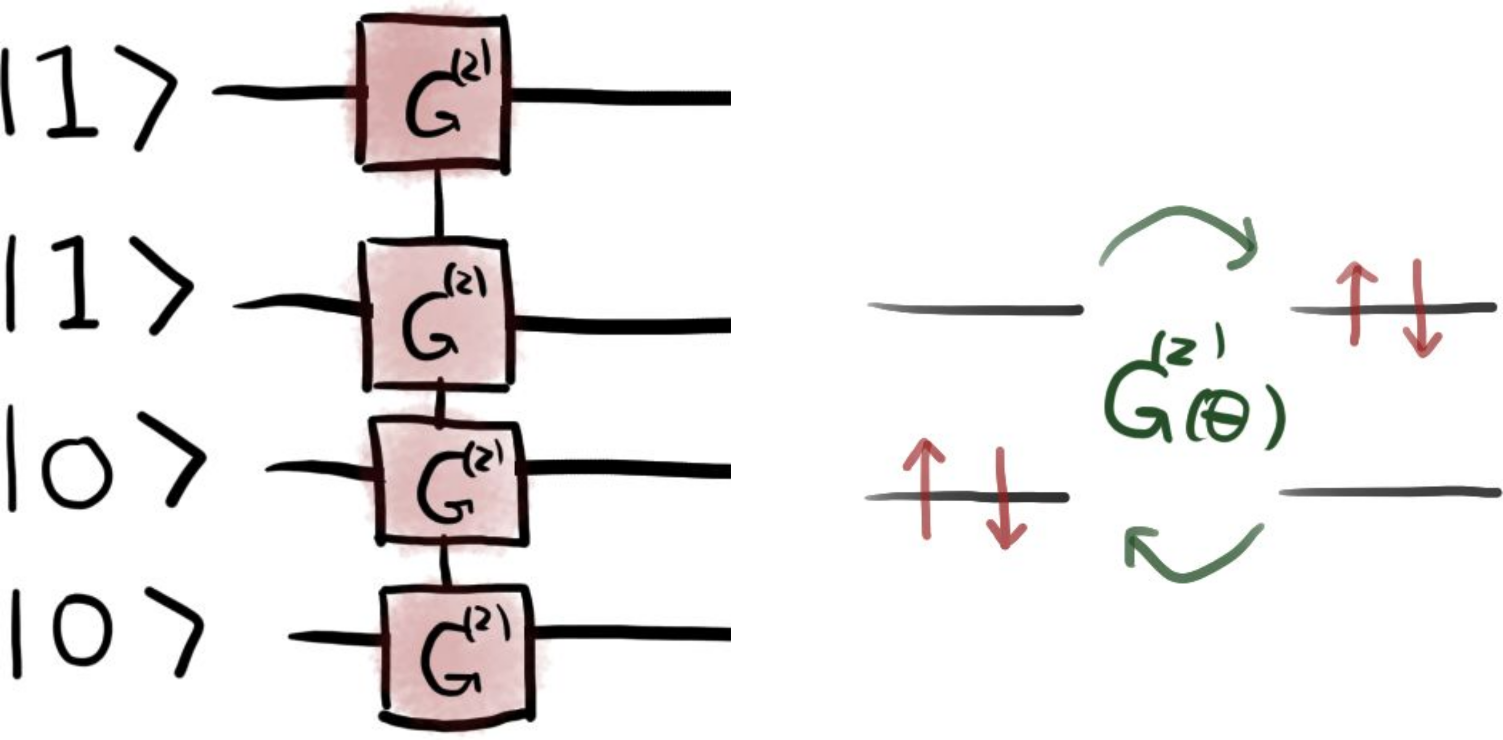
In this figure, the gate \(G^{(2)}\) corresponds to the DoubleExcitation operation, implemented in PennyLane as a Givens rotation, which couples the four-qubit states \(\vert 1100 \rangle\) and \(\vert 0011 \rangle\). For more details on how to use the excitation operations to build quantum circuits for quantum chemistry applications see the tutorial Givens rotations for quantum chemistry.

Implementing the circuit above using PennyLane is straightforward. First, we use the hf_state() function to generate the vector representing the Hartree-Fock state.

electrons = 2
hf = qml.qchem.hf_state(electrons, qubits)
print(hf)

Out:

[1 1 0 0]

The hf array is used by the BasisState operation to initialize the qubit register. Then, we just act with the DoubleExcitation operation on the four qubits.

def circuit(param, wires):
    qml.BasisState(hf, wires=wires)
    qml.DoubleExcitation(param, wires=[0, 1, 2, 3])

The next step is to define the cost function to compute the expectation value of the molecular Hamiltonian in the trial state prepared by the circuit. We do this using the expval() function. The decorator syntax allows us to run the cost function as an executable QNode with the gate parameter \(\theta\):

@qml.qnode(dev, interface="autograd")
def cost_fn(param):
    circuit(param, wires=range(qubits))
    return qml.expval(H)

Now we proceed to minimize the cost function to find the ground state of the \(\mathrm{H}_2\) molecule. To start, we need to define the classical optimizer. PennyLane offers many different built-in optimizers. Here we use a basic gradient-descent optimizer.

opt = qml.GradientDescentOptimizer(stepsize=0.4)

We initialize the circuit parameter \(\theta\) to zero, meaning that we start from the Hartree-Fock state.

theta = np.array(0.0, requires_grad=True)

We carry out the optimization over a maximum of 100 steps aiming to reach a convergence tolerance of \(10^{-6}\) for the value of the cost function.

# store the values of the cost function
energy = [cost_fn(theta)]

# store the values of the circuit parameter
angle = [theta]

max_iterations = 100
conv_tol = 1e-06

for n in range(max_iterations):
    theta, prev_energy = opt.step_and_cost(cost_fn, theta)

    energy.append(cost_fn(theta))
    angle.append(theta)

    conv = np.abs(energy[-1] - prev_energy)

    if n % 2 == 0:
        print(f"Step = {n},  Energy = {energy[-1]:.8f} Ha")

    if conv <= conv_tol:
        break

print("\n" f"Final value of the ground-state energy = {energy[-1]:.8f} Ha")
print("\n" f"Optimal value of the circuit parameter = {angle[-1]:.4f}")

Out:

Step = 0,  Energy = -1.12799983 Ha
Step = 2,  Energy = -1.13466246 Ha
Step = 4,  Energy = -1.13590595 Ha
Step = 6,  Energy = -1.13613667 Ha
Step = 8,  Energy = -1.13617944 Ha
Step = 10,  Energy = -1.13618736 Ha
Step = 12,  Energy = -1.13618883 Ha

Final value of the ground-state energy = -1.13618883 Ha

Optimal value of the circuit parameter = 0.2089

Let’s plot the values of the ground state energy of the molecule and the gate parameter \(\theta\) as a function of the optimization step.

import matplotlib.pyplot as plt

fig = plt.figure()
fig.set_figheight(5)
fig.set_figwidth(12)

# Full configuration interaction (FCI) energy computed classically
E_fci = -1.136189454088

# Add energy plot on column 1
ax1 = fig.add_subplot(121)
ax1.plot(range(n + 2), energy, "go", ls="dashed")
ax1.plot(range(n + 2), np.full(n + 2, E_fci), color="red")
ax1.set_xlabel("Optimization step", fontsize=13)
ax1.set_ylabel("Energy (Hartree)", fontsize=13)
ax1.text(0.5, -1.1176, r"$E_\mathrm{HF}$", fontsize=15)
ax1.text(0, -1.1357, r"$E_\mathrm{FCI}$", fontsize=15)
plt.xticks(fontsize=12)
plt.yticks(fontsize=12)

# Add angle plot on column 2
ax2 = fig.add_subplot(122)
ax2.plot(range(n + 2), angle, "go", ls="dashed")
ax2.set_xlabel("Optimization step", fontsize=13)
ax2.set_ylabel("Gate parameter $\\theta$ (rad)", fontsize=13)
plt.xticks(fontsize=12)
plt.yticks(fontsize=12)

plt.subplots_adjust(wspace=0.3, bottom=0.2)
plt.show()

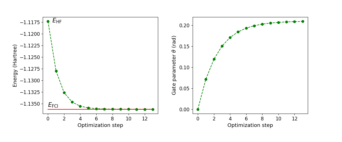
In this case, the VQE algorithm converges after thirteen iterations. The optimal value of the circuit parameter \(\theta^* = 0.208\) defines the state

\[\vert \Psi(\theta^*) \rangle = 0.994~\vert 1100 \rangle - 0.104~\vert 0011 \rangle,\]

which is precisely the ground state of the \(\mathrm{H}_2\) molecule in a minimal basis set approximation.

Conclusion

In this tutorial, we have implemented the VQE algorithm to find the ground state of the hydrogen molecule. We used a simple circuit to prepare quantum states of the molecule beyond the Hartree-Fock approximation. The ground-state energy was obtained by minimizing a cost function defined as the expectation value of the molecular Hamiltonian in the trial state.

The VQE algorithm can be used to simulate other chemical phenomena. In the tutorial tutorial_vqe_bond_dissociation, we use VQE to explore the potential energy surface of molecules to simulate chemical reactions. Another interesting application is to probe the lowest-lying states of molecules in specific sectors of the Hilbert space. For example, see the tutorial VQE in different spin sectors. Furthermore, the algorithm presented here can be generalized to find the equilibrium geometry of a molecule as it is demonstrated in the tutorial Optimization of molecular geometries.

References

1

Alberto Peruzzo, Jarrod McClean et al., “A variational eigenvalue solver on a photonic quantum processor”. Nature Communications 5, 4213 (2014).

2(1,2)

Jacob T. Seeley, Martin J. Richard, Peter J. Love. “The Bravyi-Kitaev transformation for quantum computation of electronic structure”. Journal of Chemical Physics 137, 224109 (2012).

About the author

Alain Delgado

Alain Delgado Gran is a senior quantum scientist working at Xanadu. He has a background in quantum many-body systems and electronic structure methods. His work focuses on the application of quantum algorithms for simulating advanced materials.

demos/tutorial_vqe

 

Download Python script

 

Download Notebook

 

View on GitHub