Resource estimation for quantum chemistry

Author: Soran Jahangiri — Posted: 21 November 2022.

Quantum algorithms such as quantum phase estimation (QPE) and the variational quantum eigensolver (VQE) are widely studied in quantum chemistry as potential avenues to tackle problems that are intractable for conventional computers. However, we currently do not have quantum computers or simulators capable of implementing large-scale versions of these algorithms. This makes it difficult to properly explore their accuracy and efficiency for problem sizes where the actual advantage of quantum algorithms can potentially occur. Despite these difficulties, it is still possible to perform resource estimation to assess what we need to implement such quantum algorithms.

In this demo, we describe how to use PennyLane’s resource estimation functionality to estimate the total number of logical qubits and gates required to implement the QPE algorithm for simulating molecular Hamiltonians represented in first and second quantization. We focus on non-Clifford gates, which are the most expensive to implement in a fault-tolerant setting. We also explain how to estimate the total number of measurements needed to compute expectation values using algorithms such as VQE.

Quantum Phase Estimation

The QPE algorithm can be used to compute the phase associated with an eigenstate of a unitary operator. For the purpose of quantum simulation, the unitary operator \(U\) can be chosen to share eigenvectors with a molecular Hamiltonian \(H\), for example by setting \(U = e^{-iH}\). Estimating the phase of such a unitary then permits recovering the corresponding eigenvalue of the Hamiltonian. A conceptual QPE circuit diagram is shown below.

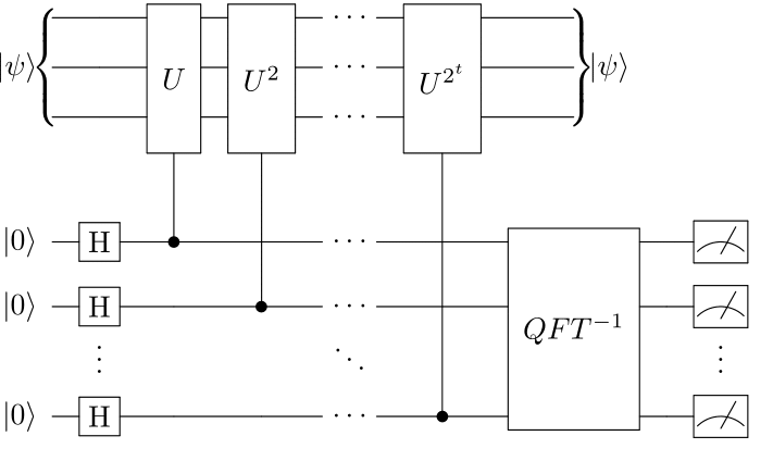
Circuit representing the quantum phase estimation algorithm.

For most cases of interest, this algorithm requires more qubits and longer circuit depths than what can be implemented on existing hardware. The PennyLane functionality in the qml.resource module allows us to estimate the number of logical qubits and the number of non-Clifford gates that are needed to implement the algorithm. We can estimate these resources by simply defining system specifications and a target error for estimation. Let’s see how!

QPE cost for simulating molecules

We study the double low-rank Hamiltonian factorization algorithm of 1 and use its cost equations as provided in APPENDIX C of 2. This algorithm requires the one- and two-electron integrals as input. These integrals can be obtained in different ways and here we use PennyLane to compute them. We first need to define the atomic symbols and coordinates for the given molecule. Let’s use the water molecule at its equilibrium geometry with the 6-31g basis set as an example.

import pennylane as qml
from pennylane import numpy as np

symbols = ['O', 'H', 'H']
geometry = np.array([[0.00000000,  0.00000000,  0.28377432],
                     [0.00000000,  1.45278171, -1.00662237],
                     [0.00000000, -1.45278171, -1.00662237]], requires_grad=False)

Then we construct a molecule object and compute the one- and two-electron integrals in the molecular orbital basis.

mol = qml.qchem.Molecule(symbols, geometry, basis_name='6-31g')
core, one, two = qml.qchem.electron_integrals(mol)()

We now create an instance of the DoubleFactorization class

algo = qml.resource.DoubleFactorization(one, two)

and obtain the estimated number of non-Clifford gates and logical qubits.

print(f'Estimated gates : {algo.gates:.2e} \nEstimated qubits: {algo.qubits}')

Out:

Estimated gates : 3.06e+08
Estimated qubits: 693

This estimation is for a target error that is set to the chemical accuracy, 0.0016 \(\text{Ha}\), by default. We can change the target error to a larger value which leads to a smaller number of non-Clifford gates and logical qubits.

chemical_accuracy = 0.0016
error = chemical_accuracy * 10
algo = qml.resource.DoubleFactorization(one, two, error=error)
print(f'Estimated gates : {algo.gates:.2e} \nEstimated qubits: {algo.qubits}')

Out:

Estimated gates : 3.06e+07
Estimated qubits: 685

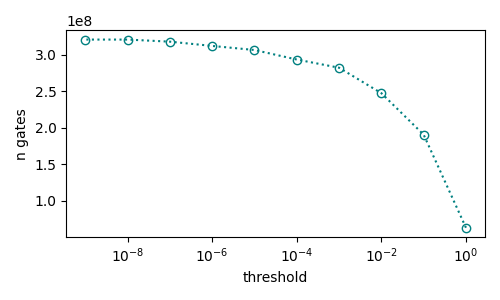
We can also estimate the number of non-Clifford gates with respect to the threshold error values for discarding the negligible factors in the factorized Hamiltonian 1 and plot the estimated numbers.

threshold = [10**-n for n in range(10)]
n_gates = []
n_qubits = []

for tol in threshold:
    algo_ = qml.resource.DoubleFactorization(one, two, tol_factor=tol, tol_eigval=tol)
    n_gates.append(algo_.gates)
    n_qubits.append(algo_.qubits)

import matplotlib.pyplot as plt

fig, ax = plt.subplots(figsize=(5, 3))
ax.plot(threshold, n_gates, ':o', markerfacecolor='none', color='teal')

ax.set_ylabel('n gates')
ax.set_xlabel('threshold')
ax.set_xscale('log')
fig.tight_layout()

QPE cost for simulating periodic materials

For periodic materials, we estimate the cost of implementing the QPE algorithm of 3 using Hamiltonians represented in first quantization and in a plane wave basis. We first need to define the number of plane waves, the number of electrons, and the volume of the unit cell that constructs the periodic material. Let’s use dilithium iron silicate \(\text{Li}_2\text{FeSiO}_4\) as an example taken from 4. For this material, the unit cell contains 156 electrons and has dimensions \(9.49 \times 10.20 \times 11.83\) in atomic units, amounting to a volume of \(1145 a_0^3\), where \(a_0\) is the Bohr radius. We also use \(10^5\) plane waves.

planewaves = 100000
electrons = 156
volume = 1145

We now create an instance of the FirstQuantization class

algo = qml.resource.FirstQuantization(planewaves, electrons, volume)

and obtain the estimated number of non-Clifford gates and logical qubits.

print(f'Estimated gates : {algo.gates:.2e} \nEstimated qubits: {algo.qubits}')

Out:

Estimated gates : 1.10e+13
Estimated qubits: 4416

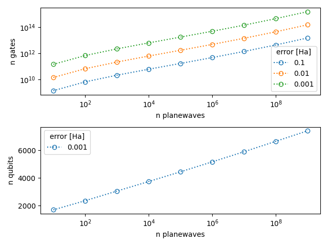
We can also plot the estimated numbers as a function of the number of plane waves for different target errors

error = [0.1, 0.01, 0.001]  # in atomic units
planewaves = [10 ** n for n in range(1, 10)]
n_gates = []
n_qubits = []

for er in error:
    n_gates_ = []
    n_qubits_ = []

    for pw in planewaves:
        algo_ = qml.resource.FirstQuantization(pw, electrons, volume, error=er)
        n_gates_.append(algo_.gates)
        n_qubits_.append(algo_.qubits)
    n_gates.append(n_gates_)
    n_qubits.append(n_qubits_)

fig, ax = plt.subplots(2, 1)

for i in range(len(n_gates)):
    ax[0].plot(planewaves, n_gates[i], ':o', markerfacecolor='none', label=error[i])
ax[1].plot(planewaves, n_qubits[i], ':o', markerfacecolor='none', label=error[-1])

ax[0].set_ylabel('n gates')
ax[1].set_ylabel('n qubits')

for i in [0, 1]:
    ax[i].set_xlabel('n planewaves')
    ax[i].tick_params(axis='x')
    ax[0].set_yscale('log')
    ax[i].set_xscale('log')
    ax[i].legend(title='error [Ha]')

fig.tight_layout()

The algorithm uses a decomposition of the Hamiltonian as a linear combination of unitaries,

\[H=\sum_{i} c_i U_i.\]

The parameter \(\lambda=\sum_i c_i\), which can be interpreted as the 1-norm of the Hamiltonian, plays an important role in determining the cost of implementing the QPE algorithm 4. In PennyLane, the 1-norm of the Hamiltonian can be obtained with

print(f'1-norm of the Hamiltonian: {algo.lamb}')

Out:

1-norm of the Hamiltonian: 649948.0644442376

PennyLane allows you to get more detailed information about the cost of the algorithms as explained in the documentation of FirstQuantization and DoubleFactorization classes.

Variational quantum eigensolver

In variational quantum algorithms such as VQE, the expectation value of an observable is typically computed by decomposing the observable into a linear combination of Pauli words, which are tensor products of Pauli and Identity operators. The expectation values are calculated through linearity by measuring the expectation value for each of these terms and combining the results. The number of qubits required for the measurement is trivially determined by the number of qubits the observable acts on. The number of gates required to implement the variational algorithm is determined by a circuit ansatz that is also known a priori. However, estimating the number of circuit evaluations, i.e. the number of shots, required to achieve a certain error in computing the expectation value is not as straightforward. Let’s now use PennyLane to estimate the number of shots needed to compute the expectation value of the water Hamiltonian.

First, we construct the molecular Hamiltonian.

H = qml.qchem.molecular_hamiltonian(symbols, geometry)[0]

The number of measurements needed to compute \(\left \langle H \right \rangle\) can be obtained with the estimate_shots() function, which requires the Hamiltonian coefficients as input. The number of measurements required to compute \(\left \langle H \right \rangle\) with a target error set to the chemical accuracy, 0.0016 \(\text{Ha}\), is obtained as follows.

m = qml.resource.estimate_shots(H.coeffs)
print(f'Shots : {m:.2e}')

Out:

Shots : 5.49e+09

This number corresponds to the measurement process where each term in the Hamiltonian is measured independently. The number can be reduced by using group_observables(), which partitions the Pauli words into groups of commuting terms that can be measured simultaneously.

ops, coeffs = qml.pauli.group_observables(H.ops, H.coeffs)

m = qml.resource.estimate_shots(coeffs)
print(f'Shots : {m:.2e}')

Out:

Shots : 2.37e+09

It is also interesting to illustrate how the number of shots depends on the target error.

error = np.array([0.02, 0.015, 0.01, 0.005, 0.001])
m = [qml.resource.estimate_shots(H.coeffs, error=er) for er in error]

e_ = np.linspace(error[0], error[-1], num=50)
m_ = 1.4e4 / np.linspace(error[0], error[-1], num=50)**2

fig, ax = plt.subplots(figsize=(5, 3))
ax.plot(error, m, 'o', markerfacecolor='none', color='teal', label='estimated')
ax.plot(e_, m_, ':', markerfacecolor='none', color='olive', label='$ 1.4e4 * 1/\epsilon^2 $')

ax.set_ylabel('shots')
ax.set_xlabel('error [Ha]')
ax.set_yscale('log')
ax.tick_params(axis='x', labelrotation = 90)
ax.legend()
fig.tight_layout()

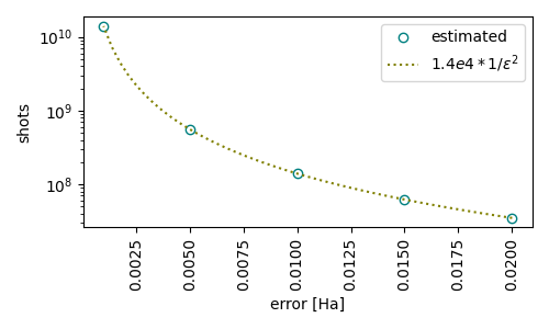
We have added a line showing the dependency of the shots to the error, as \(\text{shots} = 1.4\text{e}4 \times 1/\epsilon^2\), for comparison. Can you draw any interesting information form the plot?

Conclusions

This tutorial shows how to use the resource estimation functionality in PennyLane to compute the total number of non-Clifford gates and logical qubits required to simulate a Hamiltonian with quantum phase estimation algorithms. The estimation can be performed for second-quantized molecular Hamiltonians obtained with a double low-rank factorization algorithm, and first-quantized Hamiltonians of periodic materials in the plane wave basis. We also discussed the estimation of the total number of shots required to obtain the expectation value of an observable using the variational quantum eigensolver algorithm. The functionality allows one to obtain interesting results about the cost of implementing important quantum algorithms. For instance, we estimated the costs with respect to factors such as the target error in obtaining energies and the number of basis functions used to simulate a system. Can you think of other interesting information that can be obtained using this PennyLane functionality?

References

1(1,2)

Vera von Burg, Guang Hao Low, Thomas Haner, Damian S. Steiger, et al., “Quantum computing enhanced computational catalysis”. Phys. Rev. Research 3, 033055 (2021)

2

Joonho Lee, Dominic W. Berry, Craig Gidney, William J. Huggins, et al., “Even More Efficient Quantum Computations of Chemistry Through Tensor Hypercontraction”. PRX Quantum 2, 030305 (2021)

3

Yuan Su, Dominic W. Berry, Nathan Wiebe, Nicholas Rubin, and Ryan Babbush, “Fault-Tolerant Quantum Simulations of Chemistry in First Quantization”. PRX Quantum 2, 040332 (2021)

4(1,2)

Alain Delgado, Pablo A. M. Casares, Roberto dos Reis, Modjtaba Shokrian Zini, et al., “Simulating key properties of lithium-ion batteries with a fault-tolerant quantum computer”. Phys. Rev. A 106, 032428 (2022)

About the author

Soran Jahangiri

Soran Jahangiri is a quantum chemist working at Xanadu. His work is focused on developing and implementing quantum algorithms for chemistry applications.

demos/tutorial_resource_estimation

 

Download Python script

 

Download Notebook

 

View on GitHub