VQE with parallel QPUs with Rigetti

Author: Tom Bromley — Posted: 14 February 2020. Last updated: 9 November 2022.

This tutorial showcases how using asynchronously-evaluated parallel QPUs can speed up the calculation of the potential energy surface of molecular hydrogen (\(H_2\)).

Using a VQE setup, we task two devices from the PennyLane-Rigetti plugin with evaluating

separate terms in the qubit Hamiltonian of \(H_2\). As these devices are allowed to operate asynchronously, i.e., at the same time and without having to wait for each other, the calculation can be performed in roughly half the time.

We begin by importing the prerequisite libraries:

import time
import dask

import matplotlib.pyplot as plt
from pennylane import numpy as np
import pennylane as qml
from pennylane import qchem

This tutorial requires the pennylane-rigetti and dask packages, which are installed separately using:

pip install pennylane-rigetti
pip install "dask[delayed]"

Finding the qubit Hamiltonians of \(H_{2}\)

The objective of this tutorial is to evaluate the potential energy surface of molecular hydrogen. This is achieved by finding the ground state energy of \(H_{2}\) as we increase the bond length between the hydrogen atoms.

Each inter-atomic distance results in a different qubit Hamiltonian. To find the corresponding Hamiltonian, we use the molecular_hamiltonian() function of the qchem package. Further details on the mapping from the electronic Hamiltonian of a molecule to a qubit Hamiltonian can be found in the Building molecular Hamiltonians and A brief overview of VQE tutorials.

We begin by creating a dictionary containing a selection of bond lengths and corresponding data files saved in XYZ format. These files follow a standard format for specifying the geometry of a molecule and can be downloaded as a Zip from here.

data = {  # keys: atomic separations (in Angstroms), values: corresponding files
    0.3: "vqe_parallel/h2_0.30.xyz",
    0.5: "vqe_parallel/h2_0.50.xyz",
    0.7: "vqe_parallel/h2_0.70.xyz",
    0.9: "vqe_parallel/h2_0.90.xyz",
    1.1: "vqe_parallel/h2_1.10.xyz",
    1.3: "vqe_parallel/h2_1.30.xyz",
    1.5: "vqe_parallel/h2_1.50.xyz",
    1.7: "vqe_parallel/h2_1.70.xyz",
    1.9: "vqe_parallel/h2_1.90.xyz",
    2.1: "vqe_parallel/h2_2.10.xyz",
}

The next step is to create the qubit Hamiltonians for each value of the inter-atomic distance. We do this by first reading the molecular geometry from the external file using the read_structure() function and passing the atomic symbols and coordinates to molecular_hamiltonian().

hamiltonians = []

for separation, file in data.items():
    symbols, coordinates = qchem.read_structure(file)
    h = qchem.molecular_hamiltonian(symbols, coordinates, name=str(separation))[0]
    hamiltonians.append(h)

Each Hamiltonian can be written as a linear combination of fifteen tensor products of Pauli matrices. Let’s take a look more closely at one of the Hamiltonians:

h = hamiltonians[0]

print("Number of terms: {}\n".format(len(h.ops)))
for op in h.ops:
    print("Measurement {} on wires {}".format(op.name, op.wires))

Out:

Number of terms: 15

Measurement Identity on wires <Wires = [0]>
Measurement PauliZ on wires <Wires = [0]>
Measurement PauliZ on wires <Wires = [1]>
Measurement ['PauliZ', 'PauliZ'] on wires <Wires = [0, 1]>
Measurement ['PauliY', 'PauliX', 'PauliX', 'PauliY'] on wires <Wires = [0, 1, 2, 3]>
Measurement ['PauliY', 'PauliY', 'PauliX', 'PauliX'] on wires <Wires = [0, 1, 2, 3]>
Measurement ['PauliX', 'PauliX', 'PauliY', 'PauliY'] on wires <Wires = [0, 1, 2, 3]>
Measurement ['PauliX', 'PauliY', 'PauliY', 'PauliX'] on wires <Wires = [0, 1, 2, 3]>
Measurement PauliZ on wires <Wires = [2]>
Measurement ['PauliZ', 'PauliZ'] on wires <Wires = [0, 2]>
Measurement PauliZ on wires <Wires = [3]>
Measurement ['PauliZ', 'PauliZ'] on wires <Wires = [0, 3]>
Measurement ['PauliZ', 'PauliZ'] on wires <Wires = [1, 2]>
Measurement ['PauliZ', 'PauliZ'] on wires <Wires = [1, 3]>
Measurement ['PauliZ', 'PauliZ'] on wires <Wires = [2, 3]>

Defining the energy function

The fifteen Pauli terms comprising each Hamiltonian can conventionally be evaluated in a sequential manner: we evaluate one expectation value at a time before moving on to the next. However, this task is highly suited to parallelization. With access to multiple QPUs, we can split up evaluating the terms between the QPUs and gain an increase in processing speed.

Note

Some of the Pauli terms commute, and so they can be evaluated in practice with fewer than fifteen quantum circuit runs. Nevertheless, these quantum circuit runs can still be parallelized to multiple QPUs.

Let’s suppose we have access to two quantum devices. In this tutorial we consider two simulators from Rigetti: 4q-qvm and 9q-square-qvm, but we could also run on hardware devices from Rigetti or other providers.

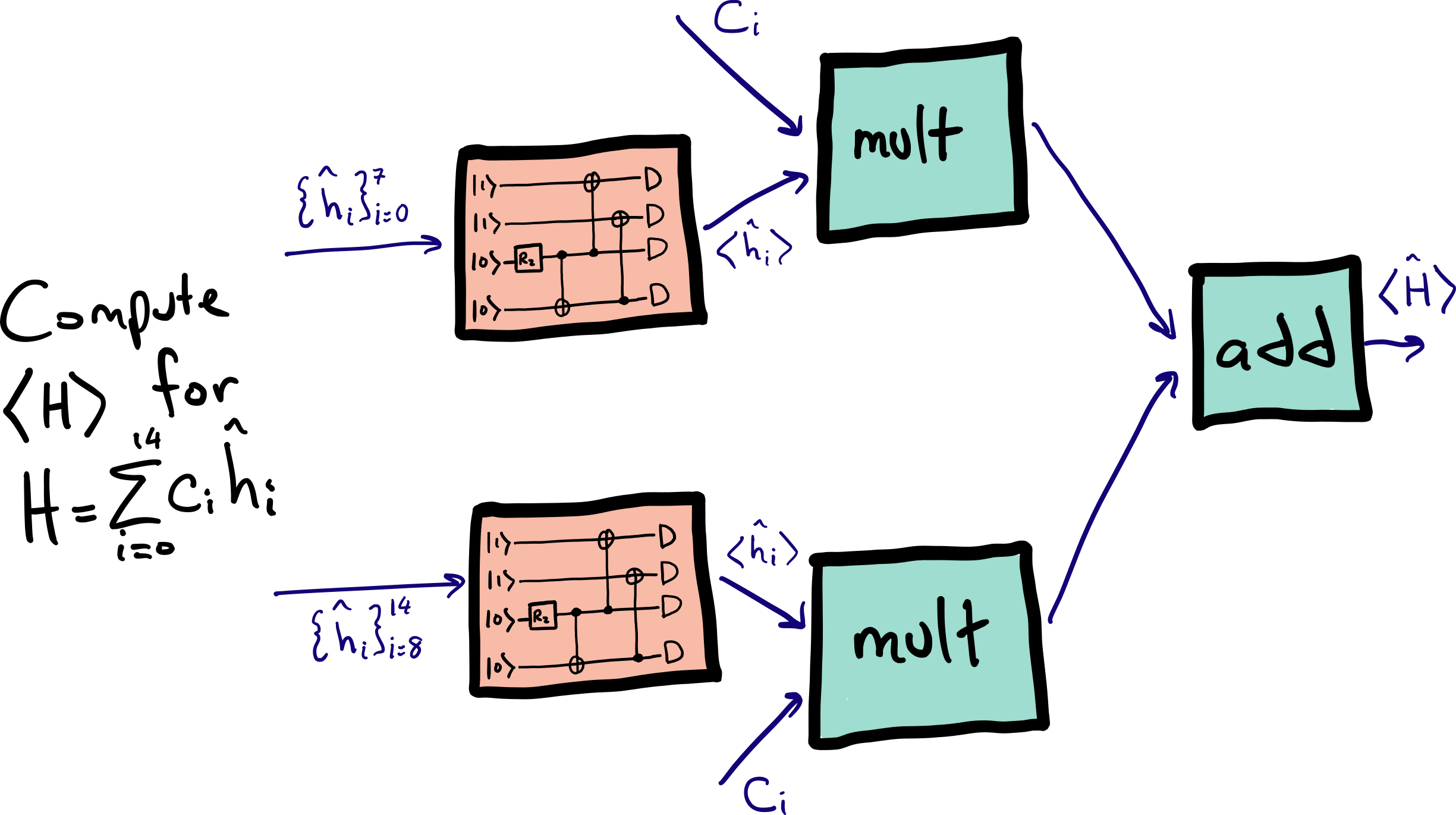
We can evaluate the expectation value of each Hamiltonian with eight terms run on one device and seven terms run on the other, as summarized by the diagram below:

To do this, start by instantiating a device for each term:

dev1 = [qml.device("rigetti.qvm", device="4q-qvm") for _ in range(8)]
dev2 = [qml.device("rigetti.qvm", device="9q-square-qvm") for _ in range(7)]
devs = dev1 + dev2

Note

For the purposes of this demonstration, we are simulating the QPUs using the rigetti.qvm simulator. To run this demonstration on hardware, simply swap rigetti.qvm for rigetti.qpu and specify the hardware device to run on.

Please refer to the Rigetti website for an up-to-date list on available QPUs.

Warning

Rigetti’s QVM and Quil Compiler services must be running for this tutorial to execute. They can be installed by consulting the Rigetti documentation or, for users with Docker, by running:

docker run -d -p 5555:5555 rigetti/quilc -R -p 5555
docker run -d -p 5000:5000 rigetti/qvm -S -p 5000

We must also define a circuit to prepare the ground state, which is a superposition of the Hartree-Fock (\(|1100\rangle\)) and doubly-excited (\(|0011\rangle\)) configurations. The simple circuit below is able to prepare states of the form \(\alpha |1100\rangle + \beta |0011\rangle\) and hence encode the ground state wave function of the hydrogen molecule. The circuit has a single free parameter, which controls a Y-rotation on the third qubit.

def circuit(param, H):
    qml.BasisState(np.array([1, 1, 0, 0], requires_grad=False), wires=[0, 1, 2, 3])
    qml.RY(param, wires=2)
    qml.CNOT(wires=[2, 3])
    qml.CNOT(wires=[2, 0])
    qml.CNOT(wires=[3, 1])
    return qml.expval(H)

The ground state for each inter-atomic distance is characterized by a different Y-rotation angle. The values of these Y-rotations can be found by minimizing the ground state energy as outlined in A brief overview of VQE. In this tutorial, we load pre-optimized rotations and focus on comparing the speed of evaluating the potential energy surface with sequential and parallel evaluation. These parameters can be downloaded by clicking here.

params = np.load("vqe_parallel/RY_params.npy")

Calculating the potential energy surface

The most vanilla execution of these 10 energy surfaces is using the standard PennyLane functionalities by executing the QNodes. Internally, this creates a measurement for each term in the Hamiltonian that are then sequentially computed.

print("Evaluating the potential energy surface sequentially")
t0 = time.time()

energies_seq = []
for i, (h, param) in enumerate(zip(hamiltonians, params)):
    print(f"{i+1} / {len(params)}: Sequential execution; Running for inter-atomic distance {list(data.keys())[i]} Å")
    energies_seq.append(qml.QNode(circuit, devs[0])(param, h))

dt_seq = time.time() - t0

print(f"Evaluation time: {dt_seq:.2f} s")

We can parallelize the individual evaluations using dask in the following way: We take the 15 terms of the Hamiltonian and distribute them to the 15 devices in devs. This evaluation is delayed using dask.delayed and later computed in parallel using dask.compute, which asynchronously executes the delayed objects in results.

def compute_energy_parallel(H, devs, param):
    assert len(H.ops) == len(devs)
    results = []

    for i in range(len(H.ops)):
        qnode = qml.QNode(circuit, devs[i])
        results.append(dask.delayed(qnode)(param, H.ops[i]))

    result = H.coeffs @ dask.compute(*results, scheduler="threads")
    return result

We can now compute all 10 samples from the energy surface sequentially, where each execution is making use of parallel device execution. Curiously, in this example the overhead from doing so outweighs the speed-up and the execution is slower than standard execution using qml.expval. For different circuits and different Hamiltonians, however, parallelization may provide significant speed-ups.

print("Evaluating the potential energy surface in parallel")
t0 = time.time()

energies_par = []
for i, (h, param) in enumerate(zip(hamiltonians, params)):
    print(f"{i+1} / {len(params)}: Parallel execution; Running for inter-atomic distance {list(data.keys())[i]} Å")
    energies_par.append(compute_energy_parallel(h, devs, param))

dt_par = time.time() - t0

print(f"Evaluation time: {dt_par:.2f} s")

We can improve this procedure further by optimizing the measurement. Currently, we are measuring each term of the Hamiltonian in a separate measurement. This is not necessary as there are sub-groups of commuting terms in the Hamiltonian that can be measured simultaneously. We can utilize the grouping function group_observables() to generate few measurements that are executed in parallel:

def compute_energy_parallel_optimized(H, devs, param):
    assert len(H.ops) == len(devs)
    results = []

    obs_groupings, coeffs_groupings = qml.pauli.group_observables(H.ops, H.coeffs, "qwc")

    for i, (obs, coeffs) in enumerate(zip(obs_groupings, coeffs_groupings)):
        H_part = qml.Hamiltonian(coeffs, obs)
        qnode = qml.QNode(circuit, devs[i])
        results.append(dask.delayed(qnode)(param, H_part))

    result = qml.math.sum(dask.compute(*results, scheduler="threads"))
    return result

print("Evaluating the potential energy surface in parallel with measurement optimization")
t0 = time.time()

energies_par_opt = []
for i, (h, param) in enumerate(zip(hamiltonians, params)):
    print(f"{i+1} / {len(params)}: Parallel execution and measurement optimization; Running for inter-atomic distance {list(data.keys())[i]} Å")
    energies_par_opt.append(compute_energy_parallel_optimized(h, devs, param))

dt_par_opt = time.time() - t0

print(f"Evaluation time: {dt_par_opt:.2f} s")

Out:

Evaluating the potential energy surface sequentially
1 / 10: Sequential execution; Running for inter-atomic distance 0.3 Å
2 / 10: Sequential execution; Running for inter-atomic distance 0.5 Å
3 / 10: Sequential execution; Running for inter-atomic distance 0.7 Å
4 / 10: Sequential execution; Running for inter-atomic distance 0.9 Å
5 / 10: Sequential execution; Running for inter-atomic distance 1.1 Å
6 / 10: Sequential execution; Running for inter-atomic distance 1.3 Å
7 / 10: Sequential execution; Running for inter-atomic distance 1.5 Å
8 / 10: Sequential execution; Running for inter-atomic distance 1.7 Å
9 / 10: Sequential execution; Running for inter-atomic distance 1.9 Å
10 / 10: Sequential execution; Running for inter-atomic distance 2.1 Å
Evaluation time: 39.33 s

Evaluating the potential energy surface in parallel
1 / 10: Parallel execution; Running for inter-atomic distance 0.3 Å
2 / 10: Parallel execution; Running for inter-atomic distance 0.5 Å
3 / 10: Parallel execution; Running for inter-atomic distance 0.7 Å
4 / 10: Parallel execution; Running for inter-atomic distance 0.9 Å
5 / 10: Parallel execution; Running for inter-atomic distance 1.1 Å
6 / 10: Parallel execution; Running for inter-atomic distance 1.3 Å
7 / 10: Parallel execution; Running for inter-atomic distance 1.5 Å
8 / 10: Parallel execution; Running for inter-atomic distance 1.7 Å
9 / 10: Parallel execution; Running for inter-atomic distance 1.9 Å
10 / 10: Parallel execution; Running for inter-atomic distance 2.1 Å
Evaluation time: 73.42 s

Evaluating the potential energy surface in parallel with measurement optimization
1 / 10: Parallel execution and measurement optimization; Running for inter-atomic distance 0.3 Å
2 / 10: Parallel execution and measurement optimization; Running for inter-atomic distance 0.5 Å
3 / 10: Parallel execution and measurement optimization; Running for inter-atomic distance 0.7 Å
4 / 10: Parallel execution and measurement optimization; Running for inter-atomic distance 0.9 Å
5 / 10: Parallel execution and measurement optimization; Running for inter-atomic distance 1.1 Å
6 / 10: Parallel execution and measurement optimization; Running for inter-atomic distance 1.3 Å
7 / 10: Parallel execution and measurement optimization; Running for inter-atomic distance 1.5 Å
8 / 10: Parallel execution and measurement optimization; Running for inter-atomic distance 1.7 Å
9 / 10: Parallel execution and measurement optimization; Running for inter-atomic distance 1.9 Å
10 / 10: Parallel execution and measurement optimization; Running for inter-atomic distance 2.1 Å
Evaluation time: 26.51 s

We have seen how Hamiltonian measurements can be parallelized and optimized at the same time.

print("Speed up: {0:.2f}".format(dt_seq / dt_par_opt))

Out:

Speed up: 1.48

To conclude the tutorial, let’s plot the calculated potential energy surfaces:

np.savez("vqe_parallel", energies_seq=energies_seq, energies_par=energies_par, energies_par_opt=energies_par_opt)

plt.plot(energies_seq, linewidth=2.2, marker="d", color="blue", label="sequential")
plt.plot(energies_par, linewidth=2.2, marker="o", color="red", label="parallel")
plt.plot(energies_par_opt, linewidth=2.2, marker="d", color="blue", label="paralell and optimized")
plt.legend(fontsize=12)
plt.title("Potential energy surface for molecular hydrogen", fontsize=12)
plt.xlabel("Atomic separation (Å)", fontsize=16)
plt.ylabel("Ground state energy (Ha)", fontsize=16)
plt.grid(True)

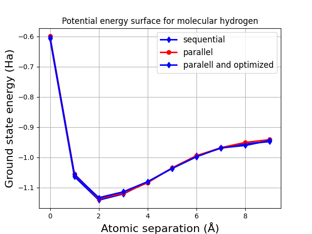
These surfaces overlap, with any variation due to the limited number of shots used to evaluate the expectation values in the rigetti.qvm device (we are using the default value of shots=1024).

About the author

Thomas Bromley

Thomas is a quantum scientist working at Xanadu. His work is focused on developing software to execute quantum algorithms on simulators and hardware.

demos/vqe_parallel

 

Download Python script

 

Download Notebook

 

View on GitHub