Quantum embedding
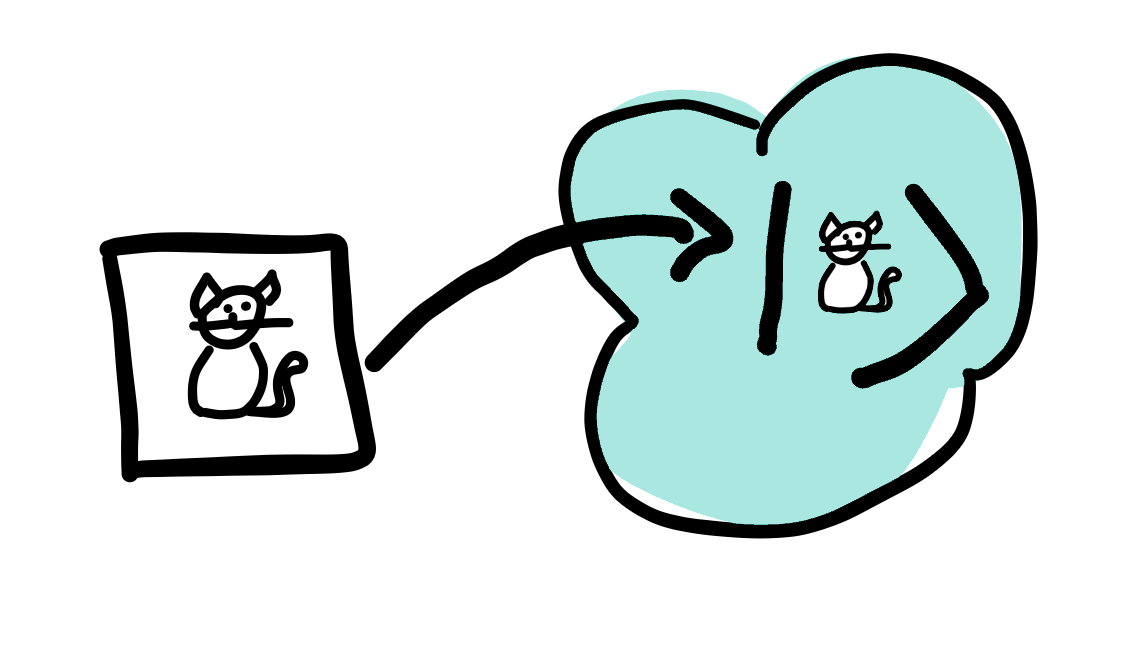
A quantum embedding represents classical data as quantum states in a Hilbert space via a quantum feature map. It takes a classical datapoint \(x\) and translates it into a set of gate parameters in a quantum circuit, creating a quantum state \(| \psi_x \rangle\). This process is a crucial part of designing quantum algorithms and affects their computational power—for more details, see Schuld & Petruccione (2018), but also Havlicek et al. (2018), Schuld & Killoran (2018), Lloyd et al. (2020).
Let’s consider classical input data consisting of \(M\) examples, with \(N\) features each,
where \(x^{(m)}\) is a \(N\)-dimensional vector for \(m=1,\ldots,M\). To embed this data into \(n\) quantum subsystems (\(n\) qubits or \(n\) qumodes for discrete- and continuous-variable quantum computing, respectively), we can use various embedding techniques, some of which are explained briefly below.
Basis Embedding
Basis embedding associates each input with a computational basis state of a qubit system. Therefore, classical data has to be in the form of binary strings. The embedded quantum state is the bit-wise translation of a binary string to the corresponding states of the quantum subsystems. For example, \(x=1001\) is represented by the 4-qubit quantum state \(| 1001 \rangle\). Hence, one bit of classical information is represented by one quantum subsystem.
Let’s consider the classical dataset \(\mathcal{D}\) mentioned above. For basis embedding, each example has to be a N-bit binary string; \(x^{(m)}=(b_1,\ldots,b_N)\) with \(b_i \in \{0,1\}\) for \(i=1,\ldots,N\). Assuming all features are represented with unit binary precision (one bit), each input example \(x^{(m)}\) can be directly mapped to the quantum state \(| x^{(m)}\rangle.\) This means that the number of quantum subsystems, \(\mathbf{n}\) , must be at least equal to \(\mathbf{N}\). An entire dataset can be represented in superpositions of computational basis states as
For example, let’s say we have a classical dataset containing two examples \(x^{(1)}=01\) and \(x^{(2)}=11\). The corresponding basis encoding uses two qubits to represent \(| x^{(1)} \rangle=|01 \rangle\) and \(| x^{(2)} \rangle=|11 \rangle\), resulting in
Note
For \(N\) bits, there are \(2^N\) possible basis states. Given \(M \ll 2^N\), the basis embedding of \(\mathcal{D}\) will be sparse.
Amplitude Embedding
In the amplitude-embedding technique, data is encoded into the amplitudes of a quantum state. A normalized classical \(N\)-dimensional datapoint \(x\) is represented by the amplitudes of a \(n\)-qubit quantum state \(| \psi_x \rangle\) as
where \(N=2^n\), \(x_i\) is the \(i\)-th element of \(x\), and \(| i \rangle\) is the \(i\)-th computational basis state. In this case, however, \(x_i\) can have different numeric data types, e.g., integer or floating point. For example, let’s say we want to encode the four-dimensional floating-point array \(x=(1.0, 0.0, -5.5, 0.0)\) using amplitude embedding. The first step is to normalize it, i.e., \(x_{norm}=\frac{1}{\sqrt{31.25}}(1.0, 0.0, -5.5, 0.0)\). The corresponding amplitude encoding uses two qubits to represent \(x_{norm}\) as
Let’s consider the classical dataset \(\mathcal{D}\) mentioned above. Its amplitude embedding can be easily understood if we concatenate all the input examples \(x^{(m)}\) together into one vector, i.e.,
where \(C_{norm}\) is the normalization constant; this vector must be normalized \(|\alpha|^2=1\). The input dataset can now be represented in the computational basis as
where \(\alpha_i\) are the elements of the amplitude vector \(\alpha\) and \(| i \rangle\) are the computational basis states. The number of amplitudes to be encoded is \(N \times M\). As a system of \(n\) qubits provides \(2^n\) amplitudes, amplitude embedding requires \(\mathbf{n \geq \log_2({NM})}\) qubits.
Note
If the total number of amplitudes to embed, i.e., \(N \times M\), is less than \(2^n\), non-informative constants can be padded to \(\alpha\) (Schuld & Petruccione (2018)).
For example, if we have 3 examples with 2 features each, we have \(3\times 2= 6\) amplitudes to embed. However, we have to use at least \(\lceil \log_2(6)\rceil = 3\) qubits, with \(2^3=8\) available states. We therefore have to concatenate \(2^3-6=2\) constants at the end of \(\alpha\).
Important
There are many other embedding techniques with similar embedding protocols. For example, squeezing embedding and displacement embedding are used with continuous-variable quantum computing models, where classical information is encoded in the squeezing and displacement operator parameters. Hamiltonian embedding uses an implicit technique by encoding information in the evolution of a quantum system (Schuld & Petruccione (2018)).
See also
PennyLane provides built-in embedding templates; see Templates for more details.
