Quantum Differentiable Programming
In quantum computing, one can automatically compute the derivatives of variational circuits with respect to their input parameters. Quantum differentiable programming is a paradigm that leverages this to make quantum algorithms differentiable, and thereby trainable.
Classical differentiable programming is a style of programming that uses automatic differentiation to compute the derivatives of functions with respect to program inputs. Differentiable programming is closely related to deep learning, but has some conceptual differences. In many early deep learning frameworks, the structure of models such as neural networks, such as the number of nodes and hidden layers, is defined statically. This is know as a “define-and-run” approach. The network is differentiable and trained using automatic differentiation and backpropagation, but the fundamental structure of the program doesn’t change.
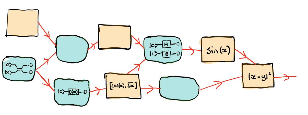
In contrast, more recent approaches use a “define-by-run” scheme, in which there is no underlying assumption to how the model is structured. The models are composed of parameterized function blocks, and the structure is dynamic—it may change depending on the input data, yet still remains trainable and differentiable. A critical aspect of this is that it holds true even in the presence of classical control flow such as for loops and if statements. These ideas allow us to use diffentiable programming in hybrid classical-quantum computations and make the entire program differentiable end-to-end.
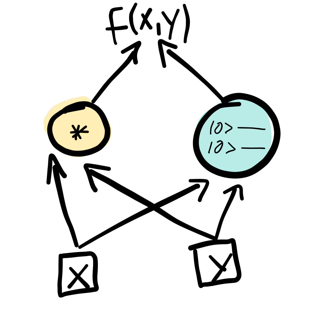
In quantum differentiable programming, hybrid computations consisting of both classical (yellow) and quantum (blue) components are automatically differentiable.
Types of differentiation in programming
Derivatives and gradients are ubiquitous throughout science and engineering. In recent years, automatic differentiation has become a key feature in many numerical software libraries, in particular for machine learning (e.g., Theano, Autograd, Tensorflow, Pytorch, or Jax).
Generally speaking, automatic differentiation is the ability for a software library to compute the derivatives of arbitrary numerical code. To better understand how it works and what the benefits are, it is instructive to analyze two other forms of differentiation that are used in software: symbolic differentation, and numerical differentiation.
Symbolic differentation
This method of differentiation is one you may be familiar with from calculus class. Symbolic differentiation manipulates expressions directly to determine the mathematical form of the gradient. Both the input and output of the procedure are mathematical expressions. For example, consider the function \(\sin(x)\). Symbolic differentiation produces
Computer algebra systems such as Mathematica perform symbolic differentiation — if you ask it for the derivative of \(\sin(x)\), it will return to you explicitly the function \(\cos(x)\), and not a numerical value. Under the hood, a set of differentiation rules are implemented and followed. This includes things like how to differentiate constants, polynomials, sums, and chain rules, as well as derivatives of common functions (e.g., trigonometric functions). This is a very powerful tool because once the set of rules is implemented, we can symbolically differentiate arbitrary functions that are encompassed by them. However the scope of this method can be limited since it requires “hand-written” support for new functions. Further, symbolic differentiation suffers from the same drawbacks we might recall from high school; sometimes, the pathway towards an analytic solution may be intensely convoluted.
Numerical differentiation
Symbolic differentation may not be always be possible when a function falls outside the set of implementated rules. It may also be very computationally complex. An alternative in these situations is to compute an approximation to the derivative numerically — this is something that can always be done. There exist a variety of such numerical methods, a common one being the finite difference method. For this method the derivative is computed by evaluating the function at two infinitesimally separated points. For example, we can approximately compute the derivative of \(\sin(x)\) as follows:
The quality of this approximation depends on the size of \(\epsilon\). A smaller \(\epsilon\) is ideal, however this can quickly cause a calculation to become unstable and can introduce floating point errors. So while numerical differentiation is always possible, it does not necessarily produce the best results for the problem at hand.
Automatic differentiation
If you write an algorithm to compute some function \(f(x, y)\) (which may
include mathematical expressions, but also control flow statements like
if, for, etc.), then automatic differentiation provides an
algorithm for computing \(\nabla f(x, y)\).
Automatic differentiation is a numerical approach, but what distinguishes it from methods like finite differences is that it is an exact method of differentiation. In a similar vein as symbolic differentiation, each component of the computation provides a rule for its derivative with respect to its inputs. However, instead of the input and output both being mathematical expressions, the output of automatic differentiation is the numerical value of the derivative.
To perform automatic differentiation, functions are first translated into computational graphs in terms of elementary operations that have known derivatives, such as addition and multiplication.
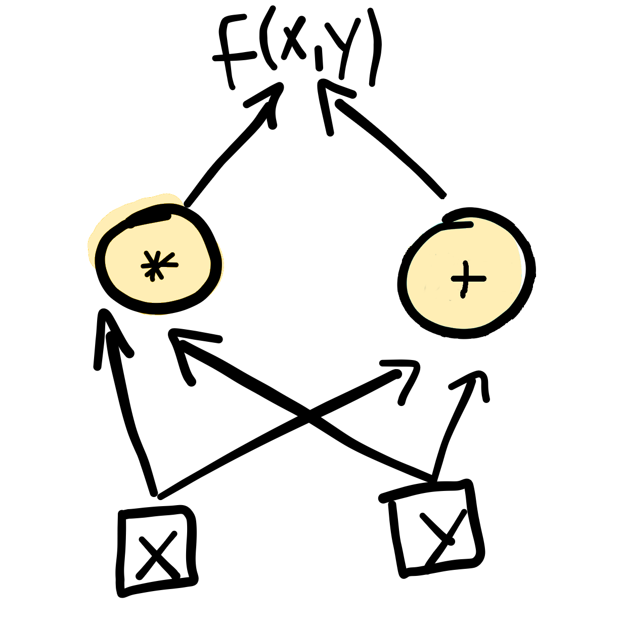
Computational graphs like this highlight the dependencies between all the parameters. To perform differentiation with respect to a particular input parameter, each node will contain information that contributes to the derivative at that point in the graph. These are then combined and propagated through using the chain rule and the differentiation rules specific to every operation. For example, nodes that perform addition and multiplication compute derivatives using the following rules:

The computational graph below shows the process for differentiating the function \(f(x, y) = xy + (x + y)\) with respect to \(x\) at the point \((x, y) = (2, 3)\). Symbolically we can compute that \(\frac{\partial f}{\partial x} = y + 1\), which gives a gradient of 4. Using automatic differentiation, the derivative with respect to \(x\) is numerically computed using the rules in the previous figure for each step of the calculation, and propagated through to produce the final result.
From this example, you can see that the computation can be arbitrarily extended
to include more nodes and variables, and different elementary operations
(provided their derivatives are known). When there is classical control flow,
such as an if statement, the computational graph branches and
gradients are only computed in the branch where the criteria is satisfied.
Note
The method of computing the gradient shown in the animation is a type of “forward-mode” autodifferentiation, since the values of the gradient are computed in the same direction of the computation. In forward-mode, the complexity of autodifferentiating a function \(f : R^m \rightarrow R\) scales with the number of parameters of the function, \(m\). There are also “backwards”, or “reverse-mode” methods, a famous one being the backpropagation used for training neural networks. In reverse-mode autodifferentiation, the gradient can be computed with the same degree of complexity as the original function, regardless of the number of parameters (albeit with some additional memory overhead).
Automatic differentiation of quantum computations
The ability to compute quantum gradients means that quantum computations can become part of automatically differentiable hybrid computation pipelines. For example, in PennyLane parameterized quantum operations carry information about their parameters and specify a “recipe” that details how to automatically compute gradients.

Many quantum operations make use of parameter-shift rules for this purpose. Parameter-shift rules are an example of forward-mode autodifferentiation, and bear some resemblance to the finite difference method presented above. They involve expressing the gradient of a function as some combination of that function at two different points. However, unlike in the finite difference methods, those two points are not infinitesimally close together, but rather quite far apart. For example,
where \(s\) is a large value, such as \(\pi/2\). The formula here comes from trigonometric identities relating \(\cos\) and \(\sin\). This not only provides us with an exact derivative, but also handles the issue of instability in finite differences that occurs when we must use a small shift.
This can be extended directly to the gradients of quantum operations and entire
quantum circuits (see, for example, the arbitrary unitary rotation
Rot which uses parameter-shift rules to compute the
derivative with respect to each of its three parameters). We simply evaluate the
circuit at two different points in parameter space. In this way, the gradient of
arbitrary sequences of parameterized gates can be computed. Once evaluated the
gradients can be fed forward into subsequent parts of a larger hybrid
computation.