Quantum gradients

The output of a variational circuit is the expectation value of a measurement observable, which can be formally written as a parameterized “quantum function” \(f(\theta)\) in the tunable parameters \(\theta = \theta_1, \theta_2, \dots\). As with any other such function, one can define partial derivatives of \(f\) with respect to its parameters.

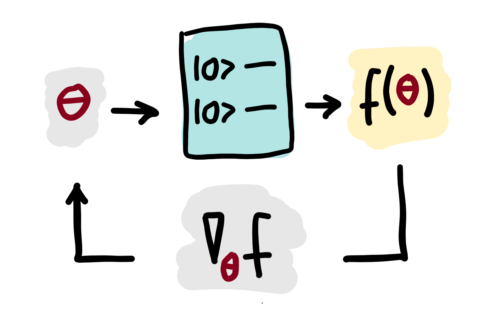
A quantum gradient is the vector of partial derivatives of a quantum function \(f(\theta)\):

\[\begin{split}\nabla_{\theta} f(\theta) = \begin{pmatrix}\partial_{\theta_1}f \\ \partial_{\theta_2} f \\ \vdots \end{pmatrix}\end{split}\]

Sometimes, quantum nodes are defined by several expectation values, for example if multiple qubits are measured. In this case, the output is described by a vector-valued function \(\vec{f}(\theta) = (f_1(\theta), f_1(\theta), ...)^T\), and the quantum gradient becomes a “quantum Jacobian”:

\[\begin{split}J_{\theta} f(\theta) = \begin{pmatrix} \partial_{\theta_1}f_1 & \partial_{\theta_1} f_2 & \dots\\ \partial_{\theta_2}f_1 & \partial_{\theta_2} f_2 & \dots\\ \vdots & & \ddots\\ \end{pmatrix}\end{split}\]

It turns out that the gradient of a quantum function \(f(\theta)\) can in many cases be expressed as a linear combination of other quantum functions via parameter-shift rules. This means that quantum gradients can be computed by quantum computers, opening up quantum computing to gradient-based optimization such as gradient descent, which is widely used in machine learning.

glossary/quantum_gradient

 

Download Python script

 

Download Notebook

 

View on GitHub