Pulse programming on Rydberg atom hardware

Author: Lillian M.A. Frederiksen — Posted: 16 May 2023.

Neutral atom hardware is a new innovation in quantum technology that has been gaining traction in recent years thanks to new developments in optical tweezer technology. One such device, QuEra’s Aquila, is capable of running circuits with up to 256 physical qubits! The Aquila device is now accessible and programmable via pulse programming in PennyLane and the PennyLane-Braket SDK plugin. In this demo, we will learn how to define a Hamiltonian for a driven Rydberg atom system in PennyLane, and use it to first simulate a pulse program on Rydberg atoms, and then upload it and measure the effect of Rydberg blockade on a hardware device!

Pulse programming basics in PennyLane

Pulse programming in PennyLane is a paradigm based on low-level control of electromagnetic driving pulses. Pulse programs are written directly on the hardware level, skipping the abstraction of decomposing algorithms into fixed native gate sets. While these abstractions are often used in proposed error correction schemes to achieve fault tolerance in a universal quantum computer, in noisy and intermediate-sized quantum computers, they can add unnecessary overhead (and thereby introduce more noise).

In quantum computing architectures where qubits are realized through physical systems with discrete energy levels, transitions from one state to another are driven by electromagnetic fields tuned to be at or near the relevant energy gap. These electromagnetic fields can vary as a function of time. The full system Hamiltonian is then a combination of the Hamiltonian describing the state of the hardware when unperturbed, and a time-dependent drive.

Pulse control gives some insight into the low-level implementation of more abstract quantum computations. In most digital quantum architectures, the native gates of the computer are, at the implementation level, electromagnetic control pulses that have been finely tuned to perform a particular logical gate.

This alternative approach requires a different type of control than what you might be used to in PennyLane, where circuits are generally defined in terms of a series of gates. Specifically, pulse control is implemented via the functionality provided in the Pennylane pulse module. For more information on pulse programming in PennyLane, see the PennyLane docs, or check out the demo about running a ctrl-VQE algorithm with pulse control on the PennyLane default.qubit simulator.

The QuEra Aquila device

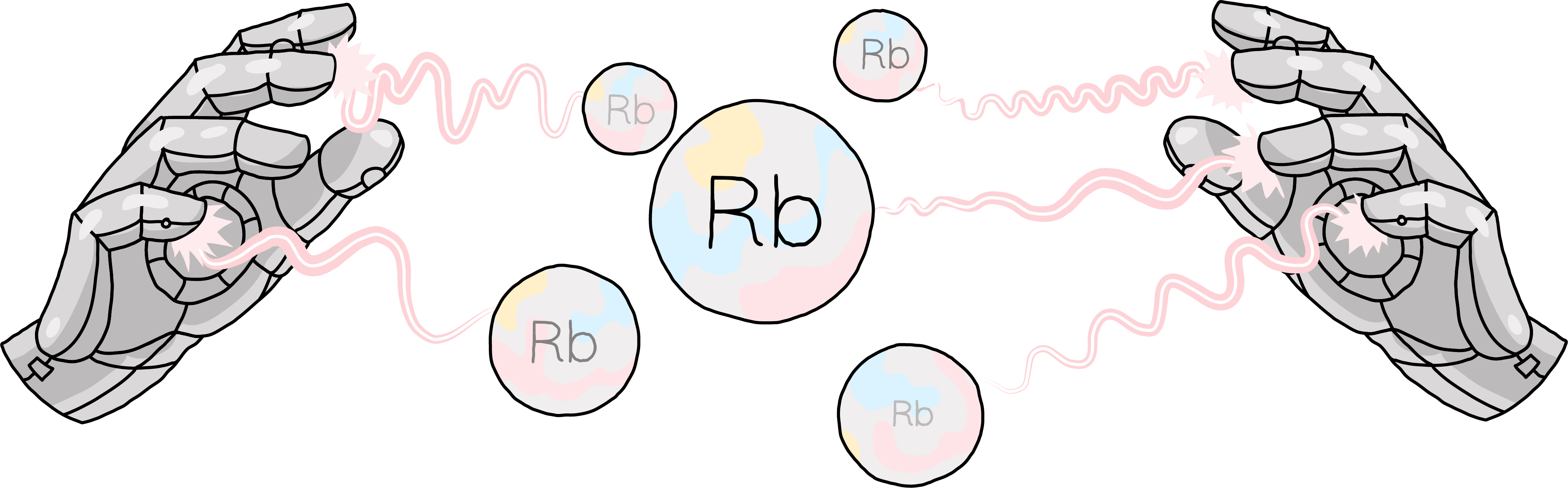
The Aquila QPU works with programmable arrays of up to 256 Rubidium-87 atoms (Rb-87), trapped in vacuum by tightly focused laser beams. These atoms can be arranged in (almost) arbitrary user-specified geometries to determine inter-qubit interactions. On the Aquila device, it is possible to specify 1D and 2D atom arrangements. Atom positions may be slightly shifted to accommodate hardware limitations, and must obey lattice constraints for spacing. This will be explored in more detail below.

Different energy levels of these atoms are used to encode qubits.

A primary application of pulse control in Rydberg atom systems like Aquila is the implementation of analog Hamiltonian simulation. This is a technique that aims to investigate the behaviour of some system of interest using a programmable, controllable device that emulates the target system. For example, Rydberg atom systems have been used to probe the behaviour of quantum spin liquids 1 and antiferromagnetic Ising models 2.

Constructing a pulse program to run on the Aquila hardware is done in two steps, each of which allows us to modify different parts of the system Hamiltonian:

1. Define atom positions, which determines qubit connectivity

2. Specify the quantum evolution via the drive parameters

Let’s start with the atom positions and the resulting Hamiltonian term describing inter-qubit interactions.

Interaction term and atom arrangement

In this treatment of the Hamiltonian, we will assume that we are operating such that we only allow access to two states; the low and high energy states are referred to as the ground (\(\ket{g}\)) and Rydberg (\(\ket{r}\)) states respectively.

Qubit interaction in a Rydberg atom system is mediated by a mechanism called Rydberg blockade, which arises due to van der Waals forces between the atoms. This is described by the interaction Hamiltonian:

\[\hat{H}_{int} = \sum_{j=1}^{N-1}\sum_{k=j+1}^{N} \frac{C_6}{R^6_{jk}}\hat{n}_j\hat{n}_k\]

where \(n_j=\ket{r_j}\bra{r_j}\) is the number operator acting on atom \(j\), \(R_{jk} = \lvert x_j - x_k \lvert\) is the distance between atoms \(j\) and \(k\), and \(C_6\) is a fixed value determined by the nature of the ground and Rydberg states (for Aquila, \(5.24 \times 10^{-24} \text{rad m}^6 / \text{s}\), referring to the \(| 70S_{1/2} \rangle\) state of the Rb-87 atom).

There are two key things to be aware of in the interaction term. First, the energy contribution of the interaction between each pair of atoms is only non-zero when both atoms are in the Rydberg state, so that \(\bra{\psi}\hat{n}_k \hat{n}_j\ket{\psi}=1\). Second, the energy contribution for each pair of atoms is inversely proportional to the distance between them. Thus, as we move two atoms closer together, it becomes increasingly energetically expensive for both to be in the Rydberg state.

In the Aquila system, to modify these interactions, we define a register (the layout of the atoms).

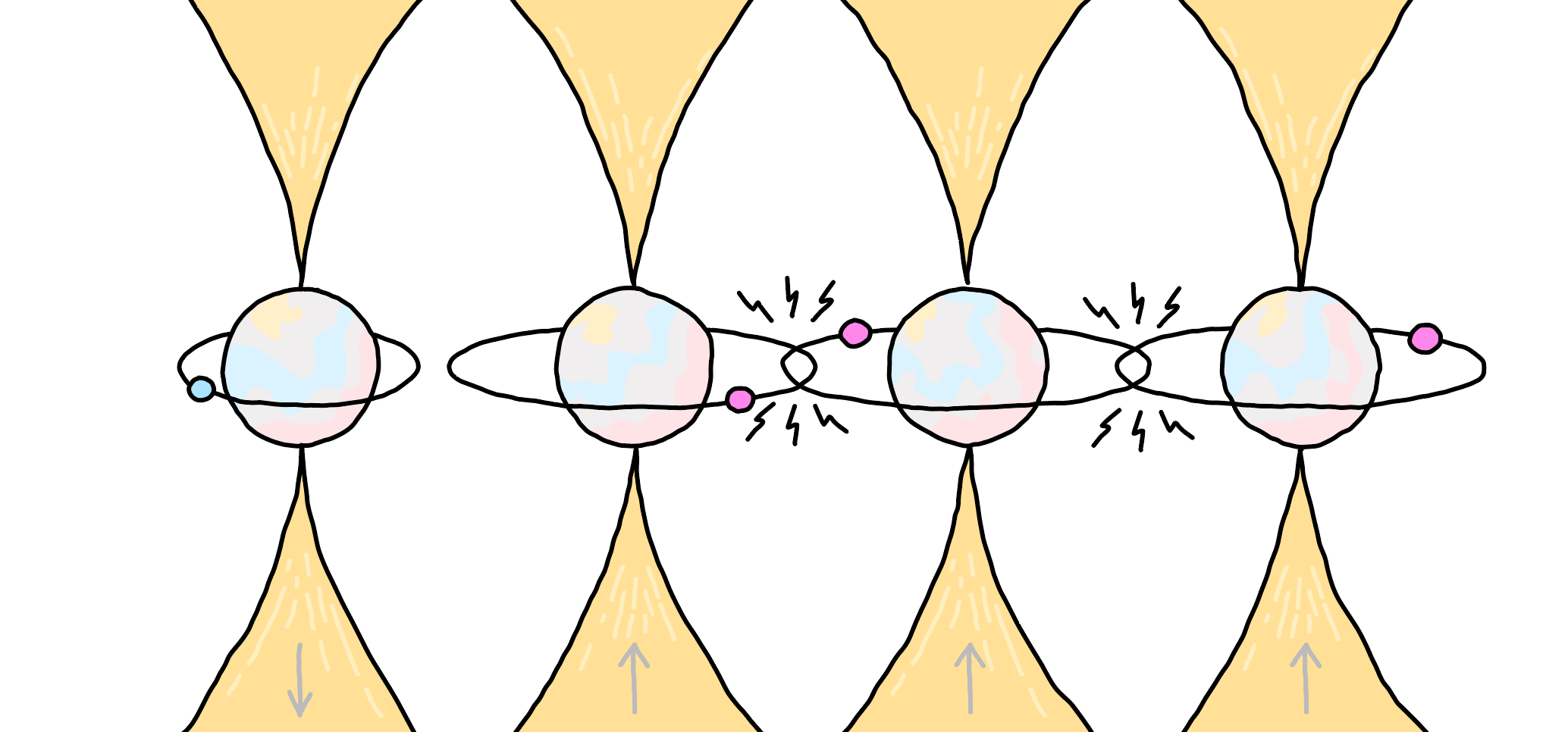
Below is a conceptual diagram demonstrating this interaction for a pair of atoms. At a distance, a similar energetic cost is paid to from 0 to 1 excitation and from 1 to 2 excitations. However, as we move the atoms into closer proximity, we see a rapidly increasing energy cost to drive to the doubly excited state.

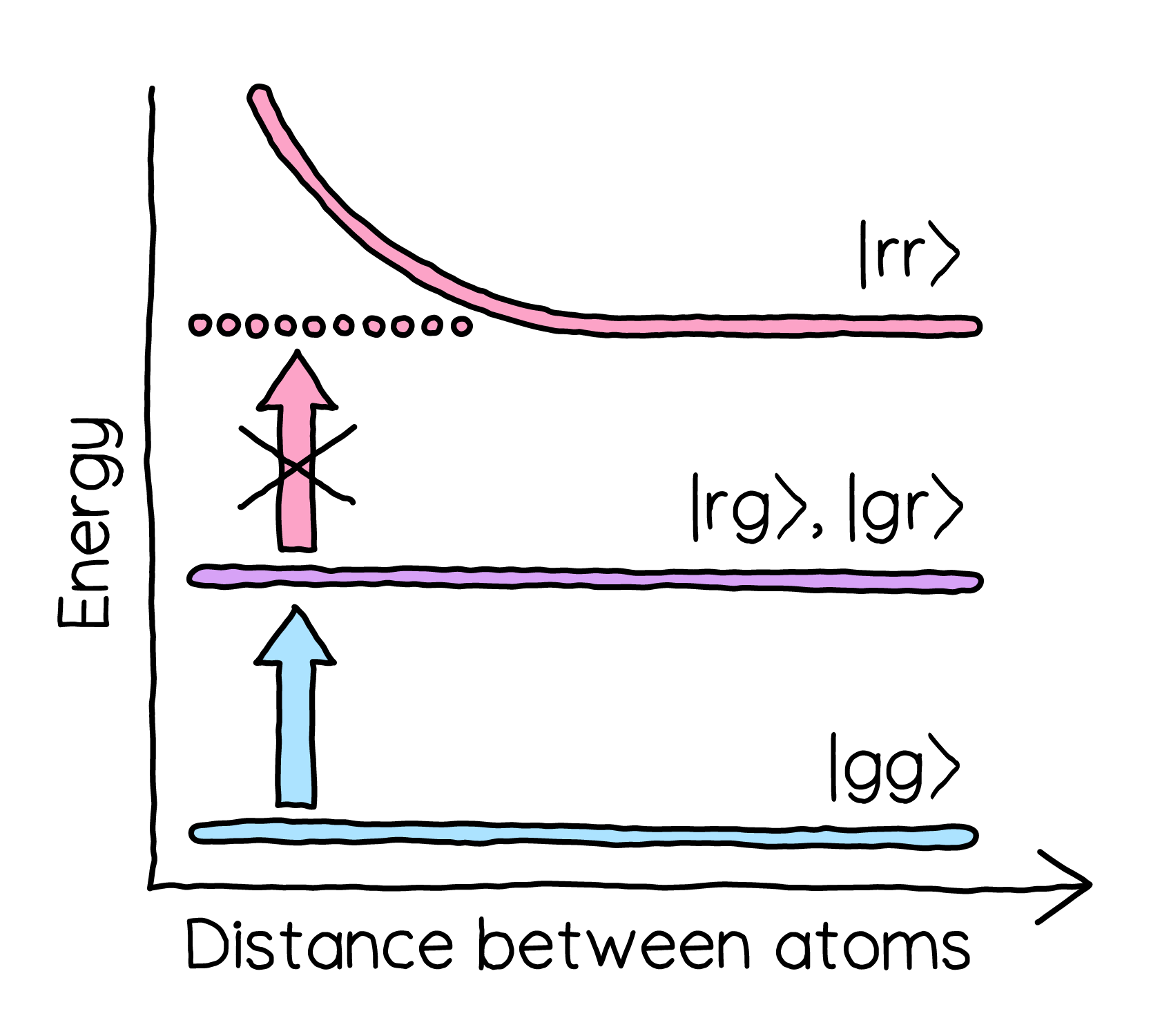
Energy levels for the ground (\(\ket{gg}\)), single Rydberg excitation (\(\ket{gr}\), \(\ket{rg}\)), and double Rydberg excitation (\(\ket{rr}\)) states

The modification of the energy levels when atoms are in proximity gives rise to Rydberg blockade, where atoms that have been driven by a pulse that would, in isolation, leave them in the excited state instead remain in the ground state due to neighboring atoms being excited.

This brings us to our discussion of the second part of the Hamiltonian: the drive term.

The driven Rydberg Hamiltonian

The atoms in a Rydberg system can be driven by application of a laser pulse, which can be described by 3 parameters: amplitude (also called Rabi frequency) \(\Omega\), detuning \(\Delta\), and phase \(\phi\). While in theory, a drive pulse can be applied to individual atoms, the current control setup for the Aquila hardware only allows the application of a global drive pulse.

Let’s look at how this plays out in the Hamiltonian describing a global drive targeting the ground to Rydberg state transition. The driven Hamiltonian of the system is:

\[\hat{H}_{drive} = \sum_{k=1}^N \frac{\Omega(t)}{2} (e^{i \phi(t)}\ket{g_k}\bra{r_k} + e^{-i \phi(t)} \ket{r_k}\bra{g_k}) - \Delta(t) \hat{n}_k\]

where \(\ket{r}\) and \(\ket{g}\) are the Rydberg and ground states.

Now that we know a bit about the system we will be manipulating, let us look at how to connect to a real device.

Getting started with Amazon Braket

For this demo, we will integrate PennyLane with Amazon Braket to perform measurements on Rydberg atom based hardware provided by QuEra.

In PennyLane, Amazon Braket is accessed through the PennyLane-Braket plugin. The installation instructions for the plugin can be found here.

The Pennylane-Braket plugin also comes pre-installed in the Braket managed notebooks accessible through the AWS console.

The remote hardware devices available on Amazon Braket can be found here, along with information about each system, including which paradigm (gate-based, continuous variable or analog Hamiltonian simulation) it operates under. Each device has a unique identifier known as an ARN. In PennyLane, AHS-based Braket devices are accessed through a PennyLane device named braket.aws.ahs, along with specification of the corresponding ARN.

Note

To access remote services on Amazon Braket, you must first create an account on AWS and also follow the setup instructions for accessing Braket from Python.

Connecting to Aquila

Once you are set up with a Braket account, you can access the Aquila device. It is available online in particular time windows, which can be found here , though you can submit tasks to the queue at any time. Note that depending on queue lengths, there can be some wait time to receive results even during the availability window of the device.

A simulated version on the Aquila hardware, braket.local.ahs, is also available, and is an excellent resource for testing out programs before committing to a particular hardware task. It is important to be aware that some tasks that succeed in simulation will not be able to be sent to hardware due to physical constraints of the measurement and control setup. Also, be aware of the hardware specifications and capabilities when planning your pulse program. These capabilities are accessible at any time from the hardware device; we will demonstrate in more detail how to access these specifications as we go through this demo.

Note

Those cells of this demo that contain the real device aquila will only run when hardware is online. If you want to run it at other times to experiment with the concepts, the hardware device can be switched out with the Braket AHS simulator. When interpreting the section of the demo regarding discretization for hardware, bear in mind that the simulator does not discretize the functions before upload, so it will not accurately demonstrate the discretization behaviour.

Let us access both the remote hardware device, and a local Rydberg atom simulator from AWS, and then we can start defining our pulse program.

import pennylane as qml

aquila = qml.device(
    "braket.aws.ahs",
    device_arn="arn:aws:braket:us-east-1::device/qpu/quera/Aquila",
    wires=3,
)

rydberg_simulator = qml.device("braket.local.ahs", wires=3)

Creating a Rydberg Hamiltonian

To create a pulse program, we first create a ParametrizedHamiltonian that describes a Rydberg system and drive we want to implement. Once created, this can be used with the default.qubit device to simulate the system’s behaviour directly in PennyLane, as well as with the AWS simulator and hardware services.

Atom layout and interaction term

Recall that placing atoms in close proximity creates a blockade effect, where it is energetically favourable for only one atom in each pair to be in the Rydberg state.

Here we define a lattice of 3 atoms, all close enough together that we would expect only one of them to be excited at a time. We can see the hardware specifications for the atom lattice via:

# units from the hardware backend are specified in SI units, in this case metres
aquila.hardware_capabilities["lattice"].dict()

Out:

{'area': {'width': Decimal('0.000075'), 'height': Decimal('0.000076')},
 'geometry': {'spacingRadialMin': Decimal('0.000004'),
  'spacingVerticalMin': Decimal('0.000004'),
  'positionResolution': Decimal('1E-7'),
  'numberSitesMax': 256}}

We can see that the atom field has a width of \(75 \, \mu m\) and a height of \(76 \, \mu m\). Additionally, we can see that the minimum radial spacing and minimal vertical spacing between two atoms are both \(4 \, \mu m\), and the resolution for atom placement is \(0.1 \, \mu m\). For more details accessing and interpreting these specifications, see Amazon Braket’s starter Aquila example notebook.

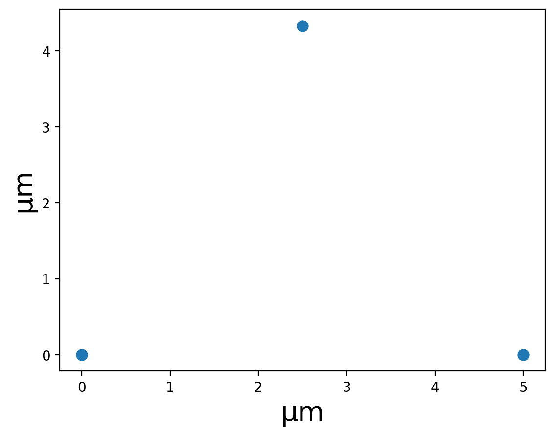
In PennyLane, we will specify these distances in micrometres. Let’s set the coordinates to be three points on an equilateral triangle with a side length of \(5 \, \mu m\), which should be well within the blockade radius:

import numpy as np
import matplotlib.pyplot as plt

a = 5

coordinates = [(0, 0), (a, 0), (a / 2, np.sqrt(a**2 - (a / 2) ** 2))]

print(f"coordinates: {coordinates}")

Out:

coordinates: [(0, 0), (5, 0), (2.5, 4.330127018922194)]

plt.scatter([x for x, y in coordinates], [y for x, y in coordinates])
plt.xlabel("μm")
plt.ylabel("μm")

If we want to create a Hamiltonian that we can use in PennyLane to accurately simulate a system, we need the correct physical constants; in this case, we need an accurate value of \(C_6\) to calculate the interaction term (different atoms and different sets of energy levels will have different physical constants). We can access these via

settings = aquila.settings
settings

Out:

{'interaction_coeff': 862619.7915580727}

PennyLane provides a helper function that creates the relevant Hamiltonian, rydberg_interaction(). We pass this function the atom coordinates, along with the settings we retrieved above, to create the interaction term for the Hamiltonian:

\[\hat{H} = \sum_{j=1}^{N-1}\sum_{k=j+1}^{N} \frac{C_6}{R^6_{jk}}\hat{n}_j\hat{n}_k\]

H_interaction = qml.pulse.rydberg_interaction(coordinates, **settings)

Driving field

The global drive is in relation to the transition between the ground and rydberg states. It is defined by 3 components: the amplitude (Rabi frequency), the phase, and the detuning. Let us consider the hardware limitations on each of these. We can access the dictionary for hardware specifications for driving the Rydberg transition just as we did for the lattice specifications above:

aquila.hardware_capabilities["rydberg"].dict()

Out:

{'c6Coefficient': Decimal('5.42E-24'),
 'rydbergGlobal': {'rabiFrequencyRange': (Decimal('0.0'),
   Decimal('15800000.0')),
  'rabiFrequencyResolution': Decimal('400.0'),
  'rabiFrequencySlewRateMax': Decimal('250000000000000.0'),
  'detuningRange': (Decimal('-125000000.0'), Decimal('125000000.0')),
  'detuningResolution': Decimal('0.2'),
  'detuningSlewRateMax': Decimal('2500000000000000.0'),
  'phaseRange': (Decimal('-99.0'), Decimal('99.0')),
  'phaseResolution': Decimal('5E-7'),
  'timeResolution': Decimal('1E-9'),
  'timeDeltaMin': Decimal('5E-8'),
  'timeMin': Decimal('0.0'),
  'timeMax': Decimal('0.000004')}}

It is important to note that these quantities are in radians per second rather than Hz where relevant, and are all in SI units. This means that for amplitude and detuning, we will need to convert from angular frequency in rad/s to standard frequency in MHz (the expected input unit in PennyLane) to understand the limits on PennyLane inputs. For example, for the largest possible detuning value specified in PennyLane should be 19.89 MHz:

def angular_SI_to_MHz(angular_SI):
    """Converts a value in rad/s or (rad/s)/s into MHz or MHz/s"""
    return angular_SI / (2 * np.pi) * 1e-6


angular_SI_to_MHz(125000000.00)

Out:

19.89436788648692

For further details on how to access the specifications and their descriptions for the device, including accessing units and more detailed descriptions, see AWS Aquila Notebook 01.

A summary of the general hardware restrictions for Rydberg drive in PennyLane’s expected units can be seen in the table below. Note that these can be subject to change, and for thoroughness it is best practice to confirm these numbers by accessing the device’s hardware_capabilities as shown above.

All values in units of frequency (amplitude and detuning) are provided here in the input units expected by PennyLane (MHz). For simulations, these numbers will be converted to angular frequency # (multiplied by \(2 \pi\)) internally as needed.

Note that when uploaded to hardware, the amplitude and detuning will be piecewise linear functions, while phase is piecewise constant. For amplitude and detuning, there is a maximum rate of change for the hardware output.

Parameter	Minimum value	Maximum value	Resolution	PWC or PWL	Maximum rate of change
Amplitude	0 MHz	2.51465 MHz	64 MHz	PWL	39788735 MHz/s
Phase	-99 rad	+99 rad	5e-7 rad	PWC	N/A
Detuning	-19.89436788 MHz	+19.89436788 MHz	3.2e-8 MHz	PWL	39788735 MHz/s

For the amplitude, there is an additional restriction that the first and last set-point in the pulse must be 0 MHz. The phase has a similar restriction for the first set-point, though the last set-point can take any value in the allowed range. There are no special restriction on the start and end points for detuning.

A few additional limitations to be aware of are:

• For hardware upload, the full pulse program must not exceed \(4 \, \mu s.\)

• The conversion from PennyLane to hardware upload will place set points every 50ns—consider this time resolution when defining pulses.

Each of the 3 parameters can either be constant for the duration of the pulse, or they can be defined by a callable, where the callable should respect the above hardware output capabilities at all time points. For an initial drive term, let’s start by defining a simple pulse with a time-dependent amplitude. Phase and detuning will both be set to 0.

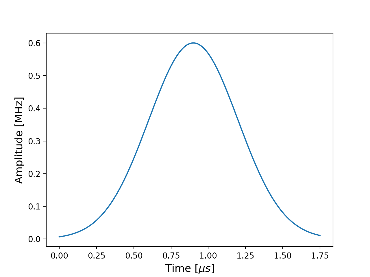
For the pulse shape, we’ll create a gaussian envelope. Because we also want to run the simulation in PennyLane, we need to define the pulse function using jax.numpy. The time is expected to be specified in microseconds for the callable.

import jax.numpy as jnp


def gaussian_fn(p, t):
    return p[0] * jnp.exp(-((t-p[1])**2) / (2*p[2]**2))


# Visualize pulse, time in μs

max_amplitude = 0.6
displacement = 0.9
sigma = 0.3

amplitude_params = [max_amplitude, displacement, sigma]

time = np.linspace(0, 1.75, 176)
y = [gaussian_fn(amplitude_params, t) for t in time]
plt.xlabel("Time [$\mu s$]")
plt.ylabel("Amplitude [MHz]")

plt.plot(time, y)

We can then define our drive using via rydberg_drive():

global_drive = qml.pulse.rydberg_drive(amplitude=gaussian_fn,
                                       phase=0,
                                       detuning=0,
                                       wires=[0, 1, 2])

With only amplitude as non-zero, the overall driven Hamiltonian in this case simplifies to:

\[\hat{H} = \sum_{k=1}^N \frac{\Omega(t)}{2} (\ket{g_k}\bra{r_k} - \ket{r_k}\bra{g_k}) + \sum_{j=1}^{N-1}\sum_{k=j+1}^{N} \frac{C_6}{R^6_{jk}}\hat{n}_j\hat{n}_k\]

Now we will use our ParametrizedHamiltonian terms to run a pulse program!

Simulating in PennyLane to find a pi-pulse

A pi-pulse is any pulse calibrated to perform a 180 degree (\(\pi\) radian) rotation on the Bloch Sphere that takes us from the ground state of the un-driven system to the excited state when applied. This corresponds to a \(\sigma_X = \ket{g}\bra{r} + \ket{r}\bra{g}\) gate in the ground-rydberg basis on each qubit. Here we will create one, and observe the effect of applying it with the interaction term “turned off”. Ignoring the inter-qubit interactions for now allows us to calibrate a pi-pulse without worrying about the effect of Rydberg blockade.

With the interaction term off, each qubit will evolve according to the unitary evolution \(U = \text{exp}\left(-i \frac{1}{2} \int d\tau \Omega(\tau) \sigma_X \right)\) and we construct \(\Omega(t)\) such that \(\int d\tau \frac{1}{2} \Omega(\tau) = \frac{\pi}{2}\), i.e. \(U = \exp(-i \frac{\pi}{2} \sigma_X) = -\sigma_X\).

We will implement the pi-pulse using the drive term defined above, and tune the parameters of the gaussian envelope to implement the desired pulse.

In the absence of the interaction term, each atom acts as a completely independent system, so we don’t see any Rydberg blockade. Below, we’ve experimented with the parameters of the gaussian pulse envelope via trial-and-error to find settings that result in a pi-pulse:

import jax

max_amplitude = 2.0
displacement = 1.0
sigma = 0.3

amplitude_params = [max_amplitude, displacement, sigma]

params = [amplitude_params]
ts = [0.0, 1.75]

default_qubit = qml.device("default.qubit.jax", wires=3, shots=1000)


@qml.qnode(default_qubit, interface="jax")
def circuit(parameters):
    qml.evolve(global_drive)(parameters, ts)
    return qml.counts()


circuit(params)

Out:

{'110': 1, '111': 999}

Simulating Rydberg blockade in PennyLane

To simulate the effect of Rydberg blockade, we create a new circuit that includes both the drive and the interaction term. We can run this simulation either in PennyLane, or using the local simulator provided by AWS:

def circuit(params):
    qml.evolve(H_interaction + global_drive)(params, ts)
    return qml.counts()


circuit_qml = qml.QNode(circuit, default_qubit, interface="jax")
circuit_ahs = qml.QNode(circuit, rydberg_simulator)

print(f"PennyLane simulation: {circuit_qml(params)}")
print(f"AWS local simulation: {circuit_ahs(params)}")

Out:

PennyLane simulation: {'000': 76, '001': 286, '010': 300, '100': 338}
AWS local simulation: {'000': 63, '001': 354, '010': 273, '100': 310}

When we apply the pi-pulse, but now to the full Hamiltonian including the interaction term, we observe that only one of the three qubits is in the excited state. This is indeed the expected effect of Rydberg blockade arising from the interaction term.

The radius within which two neighboring atoms are effectively prevented from both being excited is referred to as the blockade radius \(R_b\). The blockade radius is proportional to the \(C_6^{1/6}\) value for the transition (determining the scale of the coefficient \(V_{jk}\)). However, it is not determined by the interaction term alone-the blockade radius is also inversely proportional to how hard we drive the atoms. The blockade radius can be estimated as

\[R_b = (C_6/\sqrt{\Omega^2 + \Delta^2})^{1/6}\]

Where \(\Omega\) and \(\Delta\) describe the amplitude and detuning of the drive, respectively.

Rydberg blockade doesn’t allow neighboring atoms in close proximity to all be in the excited state.

Rydberg blockade on the QuEra hardware

Let’s look at how we would move this simple pulse program from local simulations to hardware.

Before uploading to hardware, it’s best to consider whether there are any constraints we need to be aware of. Only our amplitude parameter is non-zero, so let’s review the limitations we need to respect for defining an amplitude on hardware:

• All values must be within 0 to 2.51465 MHz

• The output will be linear between set-points, and the rate of change must never exceed 39788735 MHz/s

• The amplitude sequence must start and end at 0 MHz

times = np.linspace(0, 1.75, 1000)
amplitude = [gaussian_fn(amplitude_params, t) for t in times]

start_val = amplitude[0]
stop_val = amplitude[-1]
max_val = np.max(amplitude)
max_rate = np.max([(amplitude[i + 1] - amplitude[i]) / 50e-9 for i in range(999)])

print(f"start value: {start_val:.3} MHz")
print(f"stop value: {stop_val:.3} MHz")
print(f"maximum value: {max_val:.3} MHz")
print(f"maximum rate of change: {max_rate:.3} MHz/s")

Out:

start value: 0.00773 MHz
stop value: 0.0879 MHz
maximum value: 2.0 MHz
maximum rate of change: 1.42e+05 MHz/s

Our maximum amplitude value and maximum rate of change are well below hardware limits, so the only constraint we need to enforce for our pulse program is ensuring the values at timestamps 0 and \(1.75 \, \mu s\) are 0. For this, we can use a convenience function provided in the pulse module, rect(). We can wrap an existing function with it in order to apply a rectangular window within which the pulse has non-zero values.

Note that the function is non-zero outside the window, and the window is defined as including the end-points. This means to ensure that 0 and 1.75 return 0, they need to be outside the interval defining the window; we’ll use windows=[0.01, 1.749]. Our modified global drive is then:

amp_fn = qml.pulse.rect(gaussian_fn, windows=[0.01, 1.749])
global_drive = qml.pulse.rydberg_drive(amplitude=amp_fn,
                                       phase=0,
                                       detuning=0,
                                       wires=[0, 1, 2])

At this point we could skip directly to defining a qnode using the aquila device and running our pulse program. However, before we do, let’s take a look at how our the parameters we’ve used to define our pulse program will be converted into hardware upload data. It can be useful to examine this to ensure your pulse program looks as you expect it to before paying for a hardware run.

To do this, we create the operator we will be using in our circuit, and pass it to a method on the hardware device that creates an AHS program for upload:

op = qml.evolve(H_interaction + global_drive)(params, ts)
ahs_program = aquila.create_ahs_program(op)

On a hardware device, the create_ahs_program method will modify both the register and the pulses before upload (this method is called internally when a circuit is run on the aquila device). Float variables are rounded to specific, valid set points, producing a discretized version of the input (for example, atom locations in the register lock into grid points). For this pulse, we’re interested in the amplitude and the register.

For the register, recall that we defined our coordinates in micrometres as [(0, 0), (5, 0), (2.5, 4.330127018922194)], and that we expect the hardware upload program to be in SI units, i.e. micrometres have been converted to metres. We can access the ahs_program.register.coordinate_list to see the \(x\) and \(y\) coordinates that will be passed to hardware, and plot them against the coordinates in the register we defined for the Hamiltonian:

ahs_x_coordinates = ahs_program.register.coordinate_list(0)
ahs_y_coordinates = ahs_program.register.coordinate_list(1)

op_register = op.H.settings.register
op_x_coordinates = [x * 1e-6 for x, _ in op_register]
op_y_coordinates = [y * 1e-6 for _, y in op_register]

plt.scatter(ahs_x_coordinates, ahs_y_coordinates, label="AHS program")
plt.scatter(op_x_coordinates, op_y_coordinates, marker="x", label="Input register")
plt.xlabel("μm")
plt.ylabel("μm")
plt.legend()

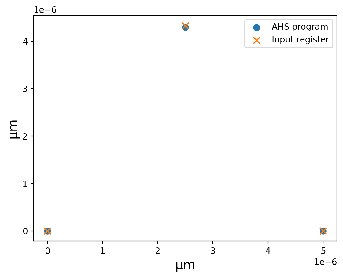
We can see that the final y-coordinate has been shifted ever so slightly when discretizing. We’re happy with this very minor change, but more intricate atom layouts, small adjustments in coordinates could have a meaningful impact in executing the program.

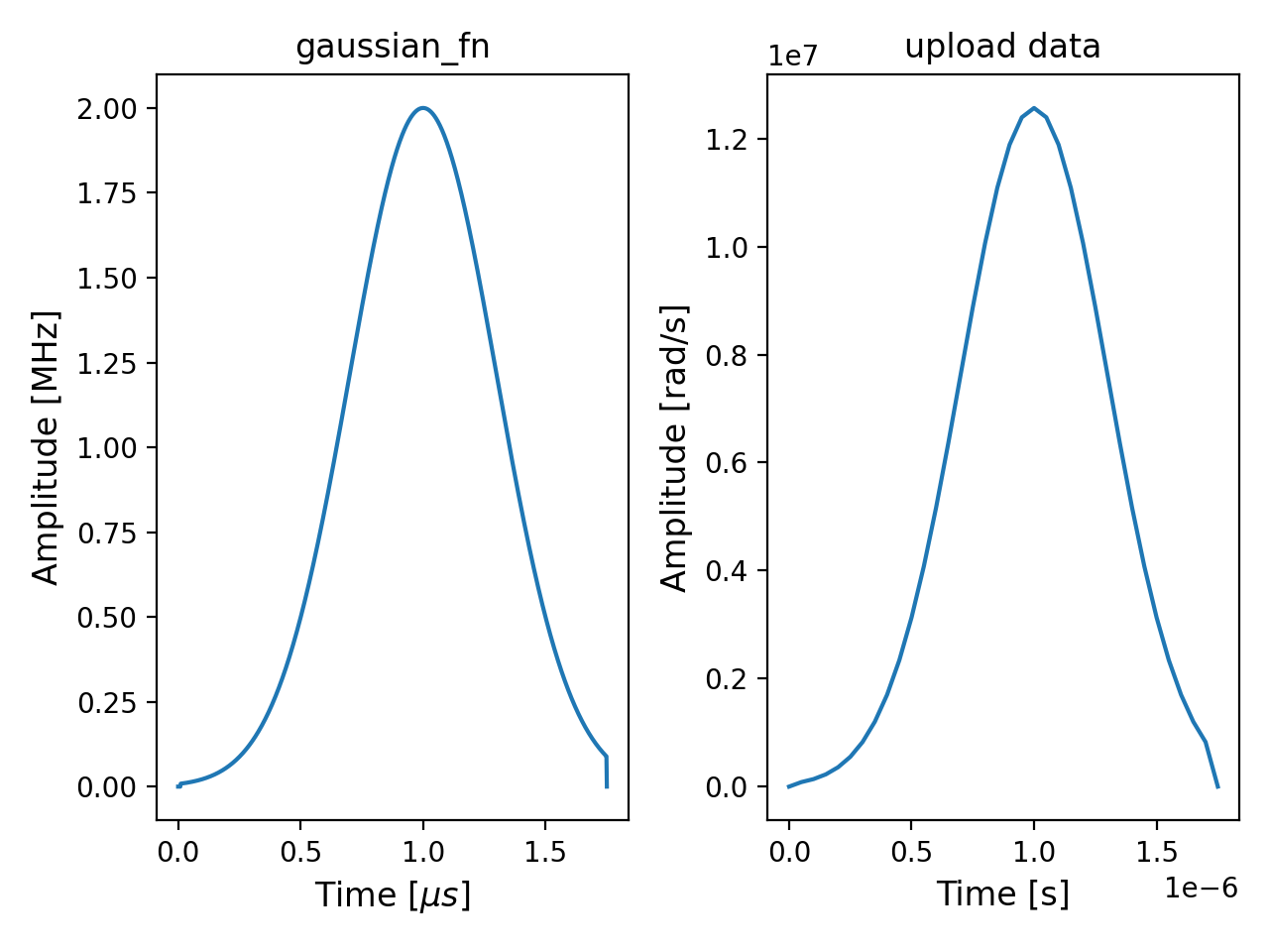
Let’s also look at the amplitude data. We can access the set-points for hardware upload from the program as ahs_program.hamiltonian.amplitude.time_series, which contains both the times() and values() for set-points. The amplitude can be switched for phase or detuning to access other relevant quantities.

# hardware set-points after conversion and discretization
amp_setpoints = ahs_program.hamiltonian.amplitude.time_series

# values for plotting the function defined in PennyLane for amplitude
input_times = np.linspace(*ts, 1000)
input_amplitudes = [
    qml.pulse.rect(gaussian_fn, windows=[0.01, 1.749])(amplitude_params, _t)
    for _t in np.linspace(*ts, 1000)
]

# plot PL input and hardware setpoints for comparison
fig, (ax1, ax2) = plt.subplots(1, 2)
ax1.plot(input_times, input_amplitudes)
ax1.set_xlabel("Time [$\mu s$]")
ax1.set_ylabel("MHz")
ax1.set_title("gaussian_fn")

ax2.plot(amp_setpoints.times(), amp_setpoints.values())
ax2.set_xlabel("Time [s]")
ax2.set_ylabel("rad/s")
ax2.set_title("upload data")

plt.tight_layout()
plt.show()

Since we are happy with this, let us send this task to hardware now. If there are any issues we’ve missed regarding ensuring the upload data is hardware compatible, we will be informed immediately. Otherwise, the task will be sent to the remote hardware; it will be run when the hardware is online and we reach the front of the queue.

To run this without connecting to the hardware, switch the aquila device out with the rydberg_simulator below. Note that running on hardware is a paid service and will incur a fee.

# @qml.qnode(rydberg_simulator)
@qml.qnode(aquila)
def circuit(params):
    qml.evolve(H_interaction + global_drive)(params, ts)
    return qml.counts()


circuit(params)

Out:

{'000': 71, '001': 296, '010': 321, '100': 312}

We observe the same pattern on the hardware that we can see in simulation—a single excitation amongst the three atoms within the blockade distance of one another. On hardware, it is possible to scale models beyond what is feasible to simulate; while simulation can’t handle large numbers of qubits, the Aquila QPU can be initialized with up to 256 qubits!

Conclusion

Rydberg atom systems are an interesting and developing field within quantum computing. It is now possible to connect to the Aquila QPU via PennyLane and Amazon Braket, and perform measurements on hardware with up to 256 qubits. Programs for the Aquila hardware can be defined using PennyLane’s pulse module, allowing users to define time-dependent control of pulse parameters.

Interfacing with the Aquila hardware provides an opportunity to take a small model of a concept that has been tested in simulation, and scale up to run on up to 256 qubits on hardware. Manipulating Rydberg atom systems through pulse-level control has applications in probing new areas of fundamental physics—like simulating quantum spin liquids at scales where it is not possible to classically simulate the quantum dynamics of the full experimental system! 1 4

Here we have demonstrated a simple, amplitude-only pulse implementing the quintessential behaviour of Rydberg atom systems: Rydberg blockade. Introducing phase and detuning to create a more complex drive Hamiltonian, and arranging atoms to create specific configurations of inter-atom interaction, allows more intricate systems to be studied.

References

1(1,2)

G. Semeghini, H. Levine, A. Keesling, S. Ebadi, T.T. Wang, D. Bluvstein, R. Verresen, H. Pichler, M. Kalinowski, R. Samajdar, A. Omran, S. Sachdev, A. Vishwanath, M. Greiner, V. Vuletic, M.D. Lukin “Probing topological spin liquids on a programmable quantum simulator” arxiv.2104.04119, 2021.

2

V. Lienhard, S. de Léséleuc, D. Barredo, T. Lahaye, A. Browaeys, M. Schuler, L.-P. Henry, A.M. Läuchli “Observing the Space- and Time-Dependent Growth of Correlations in Dynamically Tuned Synthetic Ising Models with Antiferromagnetic Interactions” arxiv.2104.04119, 2018.

3

Amazon Web Services: Amazon Braket “Hello AHS: Run your first Analog Hamiltonian Simulation” AWS Developer Guide

4

Alexander Keesling, Eric Kessler, and Peter Komar “AWS Quantum Technologies Blog: Realizing quantum spin liquid phase on an analog Hamiltonian Rydberg simulator” Amazon Quantum Computing Blog, 2021.

About the author

Lillian M.A. Frederiksen

Lillian's educational background is in experimental condensed matter physics. She has, however, traded in her cryostat for a Python IDE and is working on PennyLane as a quantum software developer at Xanadu.

demos/ahs_aquila

 

Download Python script

 

Download Notebook

 

View on GitHub