Qutrits and quantum algorithms

Author: Guillermo Alonso-Linaje — Posted: 9 May 2023. Last updated: 9 May 2023.

A qutrit is a basic quantum unit that can exist in a superposition of three possible quantum states, represented as \(|0\rangle\), \(|1\rangle\), and \(|2\rangle\), which functions as a generalization of the qubit. There are many problems to which we can apply these units, among which we can highlight an improved decomposition of the Toffoli gate. Using only qubits, it would take at least 6 CNOTs to decompose the gate, whereas with qutrits it would be enough to use 3 2. This is one of the reasons why it is important to develop the intuition behind this basic unit of information, to see where qutrits can provide an advantage. The goal of this demo is to start working with qutrits from an algorithmic point of view. To do so, we will start with the Bernstein–Vazirani algorithm, which we will initially explore using qubits, and later using qutrits.

Bernstein–Vazirani algorithm

The Bernstein–Vazirani algorithm is a quantum algorithm developed by Ethan Bernstein and Umesh Vazirani 1. It was one of the first examples that demonstrated an exponential advantage of a quantum computer over a traditional one. So, in this first section we will understand the problem that they tackled.

Suppose there is some hidden bit string “a” that we are trying to learn, and that we have access to a function \(f(\vec{x})\) that implements the following scalar product:

\[f(\vec{x}) := \vec{a}\cdot\vec{x} \pmod 2,\]

where \(\vec{a}=(a_0,a_1,...,a_{n-1})\) and \(\vec{x}=(x_0,x_1,...,x_{n-1})\) are bit strings of length \(n\) with \(a_i, x_i \in \{0,1\}\). Our challenge will be to discover the hidden value of \(\vec{a}\) by using the function \(f\). We don’t know anything about \(\vec{a}\) so the only thing we can do is to evaluate \(f\) at different points \(\vec{x}\) with the idea of gaining hidden information.

To give an example, let’s imagine that we take \(\vec{x}=(1,0,1)\) and get the value \(f(\vec{x}) = 0\). Although it may not seem obvious, knowing the structure that \(f\) has, this gives us some information about \(\vec{a}\). In this case, \(a_0\) and \(a_2\) have the same value. This is because taking that value of \(\vec{x}\), the function will be equivalent to \(a_0 + a_2 \pmod 2\), which will only take the value 0 if they are equal. I invite you to take your time to think of a possible strategy (at the classical level) in order to determine \(\vec{a}\) with the minimum number of evaluations of the function \(f\).

The optimal solution requires only \(n\) calls to the function! Let’s see how we can do this. Knowing the form of \(\vec{a}\) and \(\vec{x}\), we can rewrite \(f\) as:

\[f(\vec{x})=\sum_{i=0}^{n-1}a_ix_i \pmod 2.\]

The strategy will be to deduce one element of \(\vec{a}\) with each call to the function. Imagine that we want to determine the value \(a_i\). We can simply choose \(\vec{x}\) as a vector of all zeros except a one in the i-th position, since in this case:

\[f(\vec{x})= 0\cdot a_0 + 0\cdot a_1 + ... + 1\cdot a_i + ... + 0\cdot a_{n-1} \pmod 2 \quad= a_i.\]

It is trivial to see, therefore, that \(n\) evaluations of \(f\) are needed. The question is: can we do it more efficiently with a quantum computer? The answer is yes, and in fact, we only need to make one call to the function!

The first step is to see how we can represent this statement in a circuit. In this case, we will assume that we have an oracle \(U_f\) that encodes the function, as we can see in the picture below.

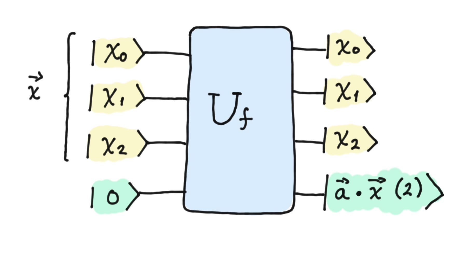
Oracle representation of the function.

In general, \(U_f\) sends the state \(|\vec{x} \rangle |y\rangle\) to the state \(| \vec{x} \rangle |y + \vec{a} \cdot \vec{x} \pmod{2} \rangle\).

Suppose, for example, that \(\vec{a}=[0,1,0]\). Then \(U_f|111\rangle |0\rangle = |111\rangle|1\rangle\), since we are evaluating \(f\) at the point \(\vec{x} = [1,1,1]\). The scalar product between the two values is \(1\), so the last qubit of the output will take the value \(1\).

The Bernstein–Vazirani algorithm makes use of this oracle according to the following circuit:

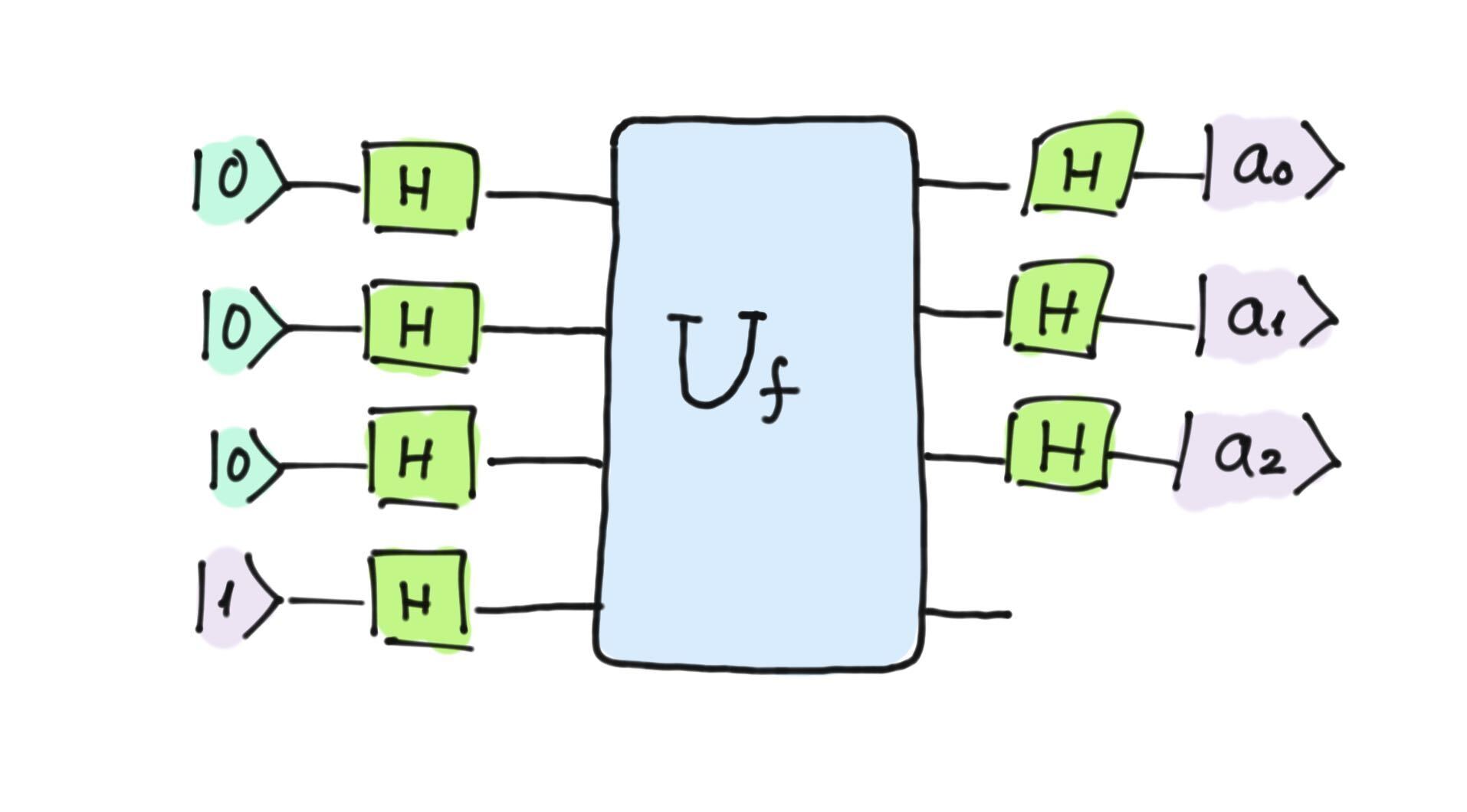
Bernstein–Vazirani algorithm.

What we can see is that, by simply using Hadamard gates before and after the oracle, after a single run, the output of the circuit is exactly the hidden value of \(\vec{a}\). Let’s do a little math to verify that this is so.

First, the input to our circuit is \(|0001\rangle\). The second step is to apply Hadamard gates to this state, and for this we must use the following property:

\[H^{\otimes n}|\vec{x}\rangle = \frac{1}{\sqrt{2^n}}\sum_{\vec{z} \in \{0,1\}^n}(-1)^{\vec{x}\cdot\vec{z}}|\vec{z}\rangle.\]

Taking as input the value \(|0001\rangle\), we obtain the state

\[|\phi_1\rangle=H^{\otimes 4}|0001\rangle = H^{\otimes 3}|000\rangle\otimes H|1\rangle = \frac{1}{\sqrt{2^3}}\left(\sum_{z \in \{0,1\}^3}|\vec{z}\rangle\right)\left(\frac{|0\rangle-|1\rangle}{\sqrt{2}}\right).\]

As you can see, we have separated the first three qubits from the fourth for clarity. If we now apply our operator \(U_f\),

\[|\phi_2\rangle= U_f |\phi_1\rangle = \frac{1}{\sqrt{2^3}}\left(\sum_{\vec{z} \in \{0,1\}^3}|\vec{z}\rangle\frac{|\vec{a}\cdot\vec{z} \pmod 2\rangle-|1 + \vec{a}\cdot\vec{z} \pmod 2\rangle}{\sqrt{2}}\right).\]

Depending on the value of \(f(\vec{x})\), the final part of the expression can take two values and it can be checked that

\[|\phi_2\rangle = \frac{1}{\sqrt{2^3}}\left(\sum_{\vec{z} \in \{0,1\}^3}|\vec{z}\rangle(-1)^{\vec{a}\cdot\vec{z}}\frac{|0\rangle-|1\rangle}{\sqrt{2}}\right).\]

This is because, if \(\vec{a}\cdot\vec{z}\) takes the value \(0\), we will have the \(\frac{|0\rangle - |1\rangle}{\sqrt{2}}\), and if it takes the value \(1\), the result will be \(\frac{|1\rangle - |0\rangle}{\sqrt{2}} = - \frac{|0\rangle - |1\rangle}{\sqrt{2}}\). Therefore, by calculating \((-1)^{\vec{a}\cdot\vec{z}}\) we cover both cases. After this, we can include the \((-1)^{\vec{a}\cdot\vec{z}}\) factor in the \(|\vec{z}\rangle\) term and disregard the last qubit, since we are not going to use it again:

\[|\phi_2\rangle =\frac{1}{\sqrt{2^3}}\sum_{\vec{z} \in \{0,1\}^3}(-1)^{\vec{a}\cdot\vec{z}}|\vec{z}\rangle.\]

Note that you cannot always disregard a qubit. In cases where there is entanglement with other qubits that is not possible, but in this case the state is separable.

Finally, we will reapply the property of the first step to calculate the result after using the Hadamard:

\[|\phi_3\rangle = H^{\otimes 3}|\phi_2\rangle = \frac{1}{2^3}\sum_{\vec{z} \in \{0,1\}^3}(-1)^{\vec{a}\cdot\vec{z}}\left(\sum_{\vec{y} \in \{0,1\}^3}(-1)^{\vec{z}\cdot\vec{y}}|\vec{y}\rangle\right).\]

Rearranging this expression, we obtain:

\[|\phi_3\rangle = \frac{1}{2^3}\sum_{\vec{y} \in \{0,1\}^3}\left(\sum_{\vec{z} \in \{0,1\}^3}(-1)^{\vec{a}\cdot\vec{z}+\vec{y}\cdot\vec{z}}\right)|\vec{y}\rangle.\]

Perfect! The only thing left to check is that, in fact, the previous state is exactly \(|\vec{a}\rangle\). It may seem complicated, but I invite you to demonstrate it by showing that \(\langle \vec{a}|\phi_3\rangle = 1\). Let’s go to the code and check that it works.

Algorithm coding with qubits

We will first code the classical solution. We will do this inside a quantum circuit to understand how to use the oracle, but we are really just programming the qubits as bits.

import pennylane as qml

dev = qml.device("default.qubit", wires = 4, shots = 1)

def Uf():
    # The oracle in charge of encoding a hidden "a" value.
    qml.CNOT(wires=[1, 3])
    qml.CNOT(wires=[2 ,3])


@qml.qnode(dev)
def circuit0():
    """Circuit used to derive a0"""


    # Initialize x = [1,0,0]
    qml.PauliX(wires = 0)

    # Apply our oracle

    Uf()

    # We measure the last qubit
    return qml.sample(wires = 3)

@qml.qnode(dev)
def circuit1():
    # Circuit used to derive a1

    # Initialize x = [0,1,0]
    qml.PauliX(wires = 1)

    # We apply our oracle
    Uf()

    # We measure the last qubit
    return qml.sample(wires = 3)

@qml.qnode(dev)
def circuit2():
    # Circuit used to derive a2
    # Initialize x = [0,0,1]
    qml.PauliX(wires = 2)

    # We apply our oracle
    Uf()

    # We measure the last qubit
    return qml.sample(wires = 3)

# We run for x = [1,0,0]
a0 = circuit0()

# We run for x = [0,1,0]
a1 = circuit1()

# We run for x = [0,0,1]
a2 = circuit2()

print(f"The value of 'a' is [{a0},{a1},{a2}]")

Out:

The value of 'a' is [0,1,1]

In this case, with 3 queries (\(n=3\)), we have discovered the value of \(\vec{a}\). Let’s run the Bernstein–Vazirani subroutine (using qubits as qubits this time) to check that one call is enough:

@qml.qnode(dev)
def circuit():

    # We initialize to |0001>
    qml.PauliX(wires = 3)

    # We run the Hadamards
    for i in range(4):
        qml.Hadamard(wires = i)

    # We apply our function
    Uf()

    # We run the Hadamards
    for i in range(3):
        qml.Hadamard(wires = i)

    # We measure the first 3 qubits
    return qml.sample(wires = range(3))

a = circuit()

print(f"The value of a is {a}")

Out:

The value of a is [0 1 1]

Great! Everything works as expected, and we have successfully executed the Bernstein–Vazirani algorithm. It is important to note that, because of how we defined our device, we are only using a single shot to find this value!

Generalization to qutrits

To make things more interesting, let’s imagine a new scenario. We are given a function of the form \(f(\vec{x}) := \vec{a}\cdot\vec{x} \pmod 3\) where, \(\vec{a}=(a_0,a_1,...,a_{n-1})\) and \(\vec{x}=(x_0,x_1,...,x_{n-1})\) are strings of length \(n\) with \(a_i, x_i \in \{0,1,2\}\). How can we minimize the number of calls to the function to discover \(\vec{a}\)? In this case, the classical procedure to detect the value of \(\vec{a}\) is the same as in the case of qubits: we will evaluate the output of the inputs \([1,0,0]\), \([0,1,0]\) and \([0,0,1]\).

But how can we work with these kinds of functions in a simple way? To do this we must use a qutrit and its operators. By using this new unit of information and unlocking the third orthogonal state, we will have states represented with a vector of dimension \(3^n\) and the operators will be \(3^n \times 3^n\) matrices where \(n\) is the number of qutrits. Specifically, we will use the TShift gate, which is equivalent to the PauliX gate for qutrits. It has the following property:

\[\text{TShift}|0\rangle = |1\rangle\]

\[\text{TShift}|1\rangle = |2\rangle\]

\[\text{TShift}|2\rangle = |0\rangle\]

This means we can use this gate to initialize each of the states. Another gate that we will use for the oracle definition is the TAdd gate, which is the generalization of the Toffoli gate for qutrits. These generalizations simply adjust the addition operation to be performed in modulo 3 instead of modulo 2. So, with these ingredients, we are ready to go to the code.

dev = qml.device("default.qutrit", wires=4, shots=1)

def Uf():
    # The oracle in charge of encoding a hidden "a" value.
    qml.TAdd(wires = [1,3])
    qml.TAdd(wires = [1,3])
    qml.TAdd(wires = [2,3])

@qml.qnode(dev)
def circuit0():

    # Initialize x = [1,0,0]
    qml.TShift(wires = 0)

    # We apply our oracle
    Uf()

    # We measure the last qutrit
    return qml.sample(wires = 3)

@qml.qnode(dev)
def circuit1():

    # Initialize x = [0,1,0]
    qml.TShift(wires = 1)

    # We apply our oracle
    Uf()

    # We measure the last qutrit
    return qml.sample(wires = 3)

@qml.qnode(dev)
def circuit2():

    # Initialize x = [0,0,1]
    qml.TShift(wires = 2)

    # We apply our oracle
    Uf()

    # We measure the last qutrit
    return qml.sample(wires = 3)

# Run to obtain the three trits of a
a0 = circuit0()
a1 = circuit1()
a2 = circuit2()


print(f"The value of a is [{a0},{a1},{a2}]")

Out:

The value of a is [0,2,1]

The question is, can we perform the same procedure as we have done before to find \(\vec{a}\) using a single shot? The Hadamard gate also generalizes to qutrits (also denoted as THadamard), so we could try to simply substitute it and see what happens!

The definition of the Hadamard gate in this space is:

\[\begin{split}\text{THadamard}=\frac{-i}{\sqrt{3}}\begin{pmatrix} 1 & 1 & 1\\ 1 & w & w^2\\ 1 & w^2 & w \end{pmatrix},\end{split}\]

where \(w = e^{\frac{2 \pi i}{3}}\). Let’s go to the code and see how to run this in PennyLane.

@qml.qnode(dev)
def circuit():

    # We initialize to |0001>
    qml.TShift(wires = 3)

    # We run the THadamard
    for i in range(4):
        qml.THadamard(wires = i)

# We run the oracle
    Uf()

# We run the THadamard again
    for i in range(3):
        qml.THadamard(wires = i)

    # We measure the first 3 qutrits
    return qml.sample(wires = range(3))

a = circuit()

print(f"The value of a is {a}")

Out:

The value of a is [0 2 1]

Awesome! The Bernstein–Vazirani algorithm generalizes perfectly to qutrits! Let’s do the mathematical calculations again to check that it does indeed make sense.

As before, the input of our circuit is \(|0001\rangle\). We will then use the Hadamard definition applied to qutrits:

\[H^{\otimes n}|\vec{x}\rangle = \frac{1}{\sqrt{3^n}}\sum_{\vec{z} \in \{0,1,2\}^n}w^{\vec{x}\cdot\vec{z}}|\vec{z}\rangle.\]

In this case, we are disregarding the global phase of \(-i\) for simplicity. Applying this to the state \(|0001\rangle\), we obtain

\[|\phi_1\rangle=H^{\otimes 4}|0001\rangle = H^{\otimes 3}|000\rangle\otimes H|1\rangle = \frac{1}{\sqrt{3^3}}\left(\sum_{z \in \{0,1,2\}^3}|\vec{z}\rangle\frac{|0\rangle+w|1\rangle+w^2|2\rangle}{\sqrt{3}}\right).\]

After that, we apply the operator \(U_f\) to obtain

\[|\phi_2\rangle= U_f |\phi_1\rangle = \frac{1}{\sqrt{3^3}}\left(\sum_{\vec{z} \in \{0,1,2\}^3}|\vec{z}\rangle\frac{|0 + \vec{a}\cdot\vec{z} \pmod 3 \rangle+w|1+ \vec{a}\cdot\vec{z} \pmod 3 \rangle+w^2|2+ \vec{a}\cdot\vec{z} \pmod 3 \rangle}{\sqrt{3}}\right).\]

Depending on the value of \(f(\vec{x})\), as before, we obtain three possible states:

• If \(\vec{a}\cdot\vec{z} = 0\), we have \(\frac{1}{\sqrt{3}}\left(|0\rangle+w|1\rangle+w^2|2\rangle\right)\).

• If \(\vec{a}\cdot\vec{z} = 1\), we have \(\frac{w^2}{\sqrt{3}}\left(|0\rangle+|1\rangle+w|2\rangle\right)\).

• If \(\vec{a}\cdot\vec{z} = 2\), we have \(\frac{w}{\sqrt{3}}\left(|0\rangle+w^2|1\rangle+|2\rangle\right)\).

Based on this, we can group the three states as \(\frac{1}{\sqrt{3}}w^{-\vec{a}\cdot\vec{z}}\left(|0\rangle+w|1\rangle+w^2|2\rangle\right)\).

After this, we can enter the coefficient in the \(|\vec{z}\rangle\) term and, as before, disregard the last qutrit, since we are not going to use it again:

\[|\phi_2\rangle =\frac{1}{\sqrt{3^3}}\sum_{\vec{z} \in \{0,1,2\}^3}w^{-\vec{a}\cdot\vec{z}}|\vec{z}\rangle.\]

Finally, we reapply the THadamard:

\[|\phi_3\rangle := H^{\otimes 3}|\phi_2\rangle = \frac{1}{3^3}\sum_{\vec{z} \in \{0,1,2\}^3}w^{-\vec{a}\cdot\vec{z}}\left(\sum_{\vec{y} \in \{0,1,2\}^3}w^{\vec{z}\cdot\vec{y}}|\vec{y}\rangle\right).\]

Rearranging this expression, we obtain:

\[|\phi_3\rangle = \frac{1}{3^3}\sum_{\vec{y} \in \{0,1,2\}^3}\left(\sum_{\vec{z} \in \{0,1,2\}^3}w^{-\vec{a}\cdot\vec{z}+\vec{y}\cdot\vec{z}}\right)|\vec{y}\rangle.\]

In the same way as before, it can be easily checked that \(\langle \vec{a}|\phi_3\rangle = 1\) and therefore, when measuring, one shot will be enough to obtain the value of \(\vec{a}\)!

Conclusion

In this demo, we have practised the use of basic qutrit gates such as TShift or THadamard by applying the Bernstein–Vazirani algorithm. In this case, the generalization has been straightforward and we have found that it makes mathematical sense, but we cannot always substitute qubit gates for qutrit gates as we have seen in the demo. To give an easy example of this, we know the property that \(X = HZH\), but it turns out that this property does not generalize! The general property is actually \(X = H^{\dagger}ZH\). In the case of qubits it holds that \(H = H^{\dagger}\), but in other dimensions it does not. I invite you to continue practising with other types of algorithms. For instance, will the Deutsch–Jozsa algorithm generalize well? Take a pen and paper and check it out!

References

1

Ethan Bernstein, Umesh Vazirani, “Quantum Complexity Theory”. SIAM Journal on Computing Vol. 26 (1997).

2

Alexey Galda, Michael Cubeddu, Naoki Kanazawa, Prineha Narang, Nathan Earnest-Noble, “Implementing a Ternary Decomposition of the Toffoli Gate on Fixed-FrequencyTransmon Qutrits”.

About the author

Guillermo Alonso-Linaje

Guillermo is a mathematics and computer science graduate from the university of Valladolid and is currently working as an educator and quantum researcher at Xanadu. Fun fact, Guillermo is a great foosball player and is also a paella master.

demos/tutorial_qutrits_bernstein_vazirani

 

Download Python script

 

Download Notebook

 

View on GitHub