Neutral-atom quantum computers

Author: Alvaro Ballon — Posted: 30 May 2023.

In the last few years, a new quantum technology has gained the attention of the quantum computing community. Thanks to recent developments in optical-tweezer technology, neutral atoms can be used as robust and versatile qubits. In 2022, a collaboration between QuEra and various academic institutions produced a neutral-atom device with a whopping 256 qubits 😲 1! It is no surprise that this family of devices has gained traction in the private sector, with startups such as Pasqal, QuEra, and Atom Computing suddenly finding themselves in the headlines.

In this tutorial, we will explore the inner workings of neutral-atom quantum devices. We will also discuss their strengths and weaknesses in terms of DiVincenzo’s criteria, introduced in the blue box below. By the end of this tutorial, you will have obtained a high-level understanding of neutral atom technologies and be able to follow the new exciting developments that are bound to come.

DiVincenzo’s criteria: In the year 2000, David DiVincenzo proposed a wishlist for the experimental characteristics of a quantum computer 2. DiVincenzo’s criteria have since become the main guideline for physicists and engineers building quantum computers:

1. Well-characterized and scalable qubits. Many of the quantum systems that we find in nature are not qubits, since we can’t just isolate two specific quantum states and tarder them. We must find a way to make them behave as such. Moreover, we need to put many of these systems together.

2. Qubit initialization. We must be able to prepare the same state repeatedly within an acceptable margin of error.

3. Long coherence times. Qubits will lose their quantum properties after interacting with their environment for a while. We need them to last long enough so that we can perform quantum operations.

4. Universal set of gates. We need to perform arbitrary operations on the qubits. To do this, we require both single-qubit gates and two-qubit gates.

5. Measurement of individual qubits. To read the result of a quantum algorithm, we must accurately measure the final state of a pre-chosen set of qubits.

We will start by explaining how neutral atoms can be manipulated and isolated enough to be used as qubits. Then, we will use PennyLane’s pulse programming capabilities to understand how to apply single and multi-qubit gates. Afterwards, we will learn how to perform measurements on the atom’s states. Finally, we will explore the work that still needs to be done to scale this technology even further.

Trapping individual atoms

In our cousin demo about trapped-ion technologies, we learn that we can trap individual charged atoms by carefully controlled electric fields. But neutral atoms, by definition, have no charge, so they can’t be affected by electric fields. How can we even hope to manipulate them individually? It turns out that the technology to do this has been around for decades 3. Optical tweezers—highly focused laser beams—can grab small objects and hold them in place, no need to charge them! Let’s see how they are able to do this.

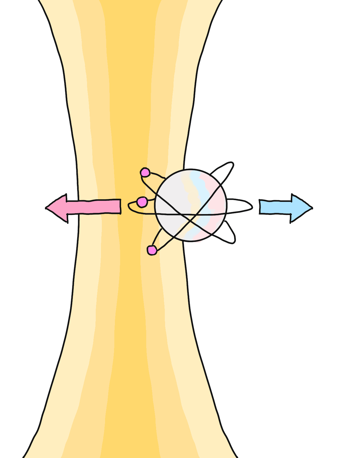
Laser beams are nothing but electromagnetic waves, that is, oscillating electric and magnetic fields. It would seem that a neutral atom could not be affected by them—but it can! To understand how, we need to keep in mind two facts. First, in a laser beam, light is more intense at the center of the beam and it dims progressively as we go toward the edges. This means that the average strength of the electric fields is higher closer to the center of the beam. Secondly, as small as neutral atoms are, they’re not just points. They do carry charges that can move around relative to each other when we expose them to electric fields.

The consequence of these two observations is that, if an atom inside a laser beam tries to escape toward the edge of the beam, the negative charges will be pulled toward the center of the beam, while the positive charges are pushed away. But, since the electric fields are stronger toward the center, the negative charges are pulled harder, so more will accumulate in the center. These negative charges will bring the positive charge that’s trying to pull away back to the middle. You can look at the figure below to gain a bit more intuition.

Electric and magnetic fields are more effective in atoms that are larger in size and whose electrons can reach high energy levels. Atoms with these features are known as Rydberg atoms and, as we will see later, their extra sensitivity to electric fields is also necessary to implemenent some quantum gates.

In the last decade, optical tweezer technology has evolved to the point where we can move atoms around into customizable arrays (check out this tutorial and have some fun doing this!). This means that we have a lot of freedom in how and when our atom-encoded qubits interact with each other. Sounds like a dream come true! However, there are some big challenges to address—we’ll learn about these later. To get started, let’s understand how neutral atoms can be used as qubits.

Encoding a qubit in an atom

To encode a qubit in a neutral atom, we need to have access to two distinct atomic quantum states. The most easily accessible quantum states in an atom are the electronic energy states. We would like to switch one electron between two different energy states, which means that we must make sure not to affect other electrons when we manipulate the atom. For this reason, the ideal atoms to work with are those with one valence electron, i.e. one “loose” electron that is not too tightly bound to the nucleus.

Note

In some cases, such as the devices built by Atom Computing 4, qubits are not encoded in atomic energy levels, but in so-called nuclear-spin energy levels instead. Such qubits are known as nuclear spin qubits. In this demo, we will not focus on the physics of these qubits. However, similar principles to those we’ll outline in this demo for qubit preparation, control, and measurement will apply to this type of qubit.

A common choice is the Rubidium-85 atom, given that it’s a Rydberg atom commonly used in atomic physics and we have the appropriate technology to change its energy state using lasers. If you need a refresher on how we change the electronic energy levels of atoms, do take a look at the blue box below!

Atomic Physics Primer: Atoms consist of a positively charged nucleus and negative electrons around it. The electrons inhabit energy levels, which have a population limit. As the levels fill up, the electrons occupy higher and higher electronic energy states, or energy levels. But as long as there is space, electrons can change energy levels, with a preference for the lower ones. This can happen spontaneously or due to external influences.

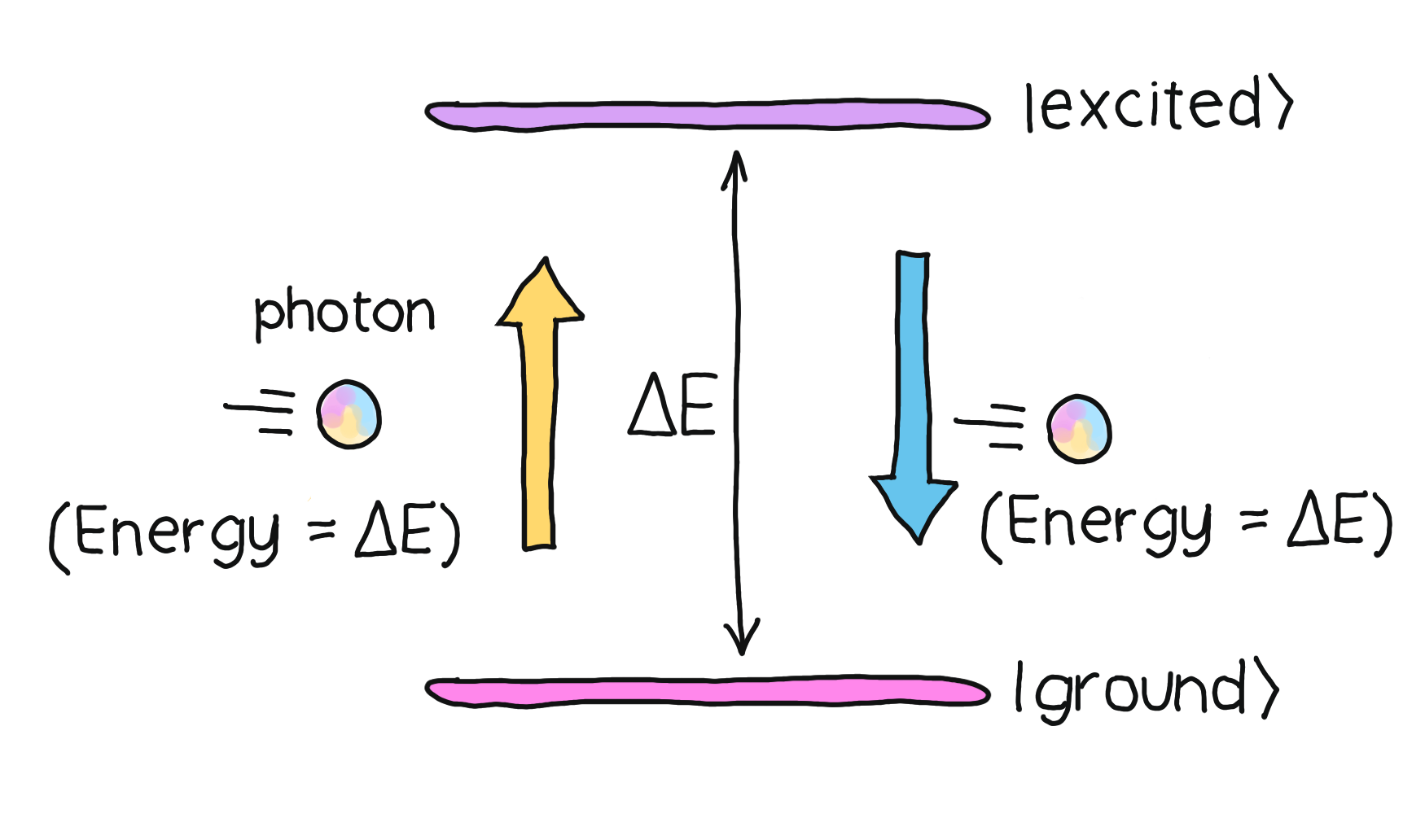
When the lower energy levels are not occupied, the higher energy levels are unstable: electrons will prefer to minimize their energy and jump to a lower level on their own. What happens when an electron jumps from a high energy level to a lower one? Conservation of energy tells us that the energy must go somewhere. Indeed, a photon with an energy equal to the energy lost by the electron is emitted. This energy is proportional to the frequency (colour) of the photon.

Conversely, we can use laser light to induce the opposite process. When an electron is in a stable or ground state, we can use lasers with their frequency set roughly to the difference in energy levels, or energy gap, between the ground state and an excited state. If a photon hits an electron, it will go to that higher energy state. When the light stimulus is removed, the excited electrons will return to stable states. The time it takes them to do so depends on the particular excited state they are in since, sometimes, the laws of physics will make it harder for electrons to jump back on their own.

But even if we’ve chosen one electron in the atom, we need to make sure that we are effectively working with only two energy levels in that atom. This ensures that we have a qubit! One of the energy levels will be a ground state for the valence electron, which we call the fiducial state and denote by \(\lvert 0 \rangle.\) The other energy level will be an long-lived excited state, known as a hyperfine state, denoted by \(\lvert 1 \rangle.\) We’ll induce transitions between these two states using light whose energy matches the energy difference between these atomic levels.

Initializing the qubits

We have chosen our atom and its energy levels, so the easy part is over! But there are still some difficult tasks ahead of us. In particular, we need to isolate individual atoms inside our optical tweezers and make sure that they are all in the fiducial ground state, as required by DiVincenzo’s second criterion. This fiducial state is stable, since minimal-energy states will not spontaneously emit any energy.

The first step to initialize the qubits is to cool down a cloud of atoms in a way that all of their electrons end up in the same state. There are many states of minimum energy, so we need to be careful that all electrons are in the same one! For Rubidium atoms, we use a technique known as laser cooling. It involves putting the atoms in a magnetic trap within a vacuum chamber and then using lasers both to freeze them in place and make sure all the electrons are in the same stable state.

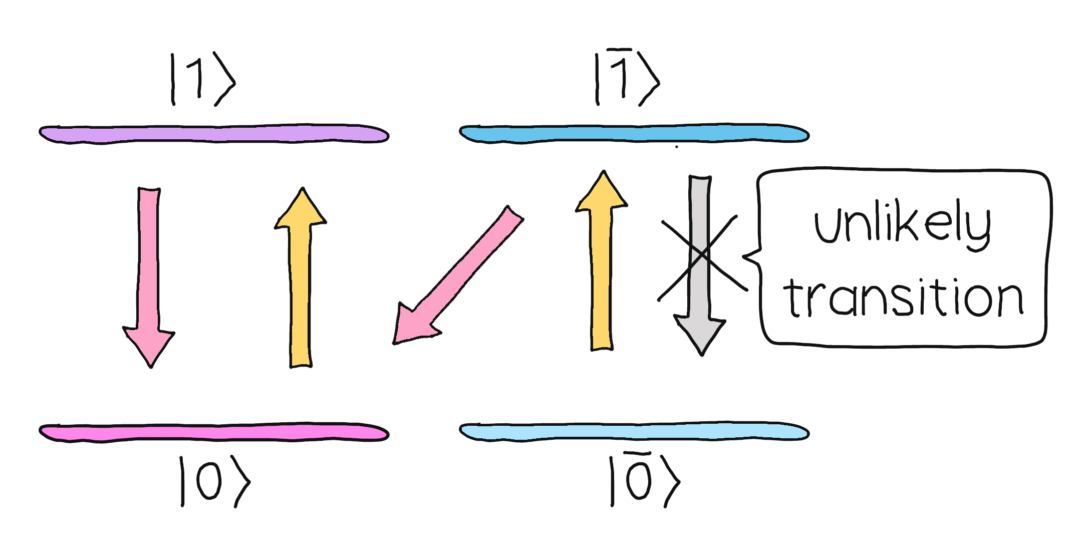
To understand how neutral atoms can be used to build a quantum device, let’s figure out how all the electrons end up in the same energy state. It turns out that Rubidium-85 is the ideal atom not only because it has one valence electron, but also because it has a closed optical loop.

Rubidium-85 has two ground states \(\vert 0\rangle\) and \(\vert \bar{0}\rangle\), which are excited using the laser to two excited states \(\vert 1\rangle\) and \(\vert \bar{1}\rangle\) respectively. However, both of these excited states will decay to \(\vert 0\rangle\) with high probability. This means that no matter what ground state the electrons occupied initially, they will most likely be driven to the same ground state through the laser cooling method.

Great! We have our cloud of atoms all frozen and in the same ground state. But now we need to pick out single atoms and arrange them in nice ways. Here’s where we use our optical tweezers. The width of the laser can be focused enough so that we are sure that at most one atom gets trapped. Moreover, one laser beam can be split into a variety of arrays of beams through a spatial light modulator, allowing us to rearrange the positions of the atoms in many ways. With our atoms in position and in the fiducial ground state, we’re ready to do some quantum operations on them!

Measuring an electronic state

Now that our fiducial state is prepared, let’s focus on another essential part of a quantum computation: measuring the state of our system. But wait… isn’t measurement the last step in a quantum circuit? Aren’t we skipping ahead a little bit? Not really! Once we have our initial state, we should measure it to verify that we have indeed prepared the correct state. After all, some of the steps we carried out to prepare the atoms aren’t really foolproof; there are two issues that we need to address.

The first problem is that traps are designed to trap at most one atom. This means that some traps might contain no atoms! With cutting-edge initialization routines, about \(2\%\) of the tweezers remain empty. The second issue is that laser cooling is not deterministic, which means that some atoms may not be in the ground state. We would like to exclude those from our initial state. Happily, there is a simple solution that addresses these two problems.

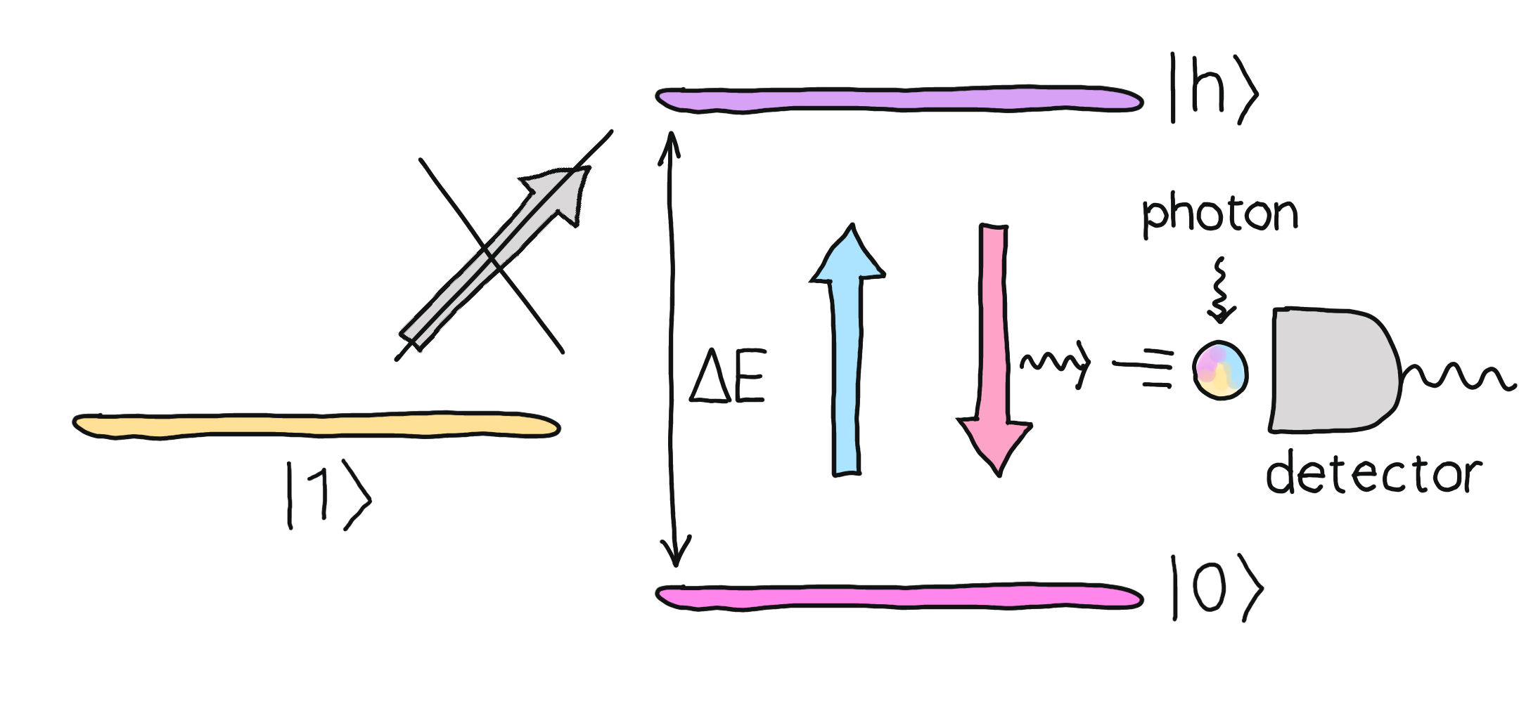
To verify that a neutral atom is in the fiducial state \(\lvert 0 \rangle\), we shine a photon on it that stimulates the transition between this state to some short-lived excited state \(\lvert h \rangle\). Electrons excited in this way will promptly decay to the state \(\lvert 0 \rangle\) again, emitting light. The electrons that are in some state different than \(\lvert 0 \rangle\) never get excited, since the photon does not have the right energy. And, of course, nothing will happen in traps where there is no atom. The net result is that atoms in the ground state will shine, while others won’t. This phenomenon, known as fluorescence, is also used in trapped ion technologies. The same method can be used at the end of a quantum computation to measure the final state of the atoms in the computational basis.

Note

What about atoms in the state \(\vert \bar{0}\rangle\)? Wouldn’t they become excited as well? We can actually choose the energy level \(\vert h\rangle\) such that the transition \(\vert \bar{0}\rangle \rightarrow \vert h\rangle\) wouldn’t conserve angular momentum, so it would be suppressed.

Neutral atoms and light

We want to carry out computations using the electronic energy levels of the neutral atoms, which means that we need to be able to control their quantum state. To do so, we need to act on it with a light pulse—a short burst of light whose amplitude and phase are carefully controlled over time. To predict exactly how pulses affect the quantum states, we need to write down the Hamiltonian of the system.

Note

Recall that the Hamiltonian \(H\) is the observable for the energy of the system, but it also describes how the system’s quantum state evolves in time. If a system’s initial state is \(\vert \psi(0)\rangle\) then, after a time interval \(t,\) the state is

\[\vert \psi(t)\rangle = \exp\left(-i\int_{0}^{t}H(\tau)d\tau\right)\vert \psi(0)\rangle.\]

In general, this is not easy to calculate. But evolve() comes to our rescue, since it will calculate \(\vert \psi(t)\rangle\) for us using some very clever approximations.

When a pulse of light of frequency \(\nu(t),\) amplitude \(\Omega(t)/2\pi\) and phase \(\phi\) is shone upon all the atoms in our array, the Hamiltonian describing this interaction turns out to be 5

\[H_d = \Omega(t)\sum_{q\in\text{wires}}(\cos(\phi)\sigma_{q}^x-\sin(\phi)\sigma_{q}^y) - \frac{1}{2}\delta(t)\sum_{q\in\text{wires}}(\mathbb{I}_q -\sigma_{q}^z).\]

Here, the detuning \(\delta(t)\) is defined as the difference between the photon’s energy and the energy \(E_{01}\) needed to transition between the ground state \(\lvert 0 \rangle\) and the excited state \(\lvert 1 \rangle:\)

\[\delta(t) = \hbar\nu(t)-E_{01}.\]

We will call \(H_d\) the drive Hamiltonian, since the electronic states of the atoms are being “driven” by the light pulse. This Hamiltonian is time-dependent, and it may also depend on other parameters that describe the pulse. PennyLane’s pennylane.pulse.ParametrizedHamiltonian class will help us deal with such a mathematical object. You can learn more about Parametrized Hamiltonians in our documentation and in this pulse Programming demo.

Driving excitations with pulses

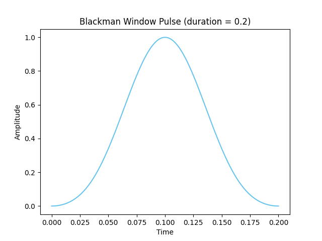
The mathematical expression of the Hamiltonian tells us that the time evolution depends on the shape of the pulse, which we can control pretty much arbitrarily as long as it’s finite in duration. We must choose a pulse shape that starts and dies off smoothly. It turns out that one of the best choices is the Blackman window pulse, which minimizes noise 6. The amplitude of a Blackman pulse of duration \(T\) is given by

\[\begin{split}\frac{\Omega(t)}{2\pi} = \left\{\begin{array}{lr} \left(\frac{1-\alpha}{2}\right)A-\frac{A}{2}\cos\left(\frac{2\pi t}{T}\right)+\frac{\alpha A}{2}\cos\left(\frac{4\pi t}{T}\right), & \text{if } 0 \leq t \leq T \\ 0 & \text{otherwise.} \end{array}\right.\end{split}\]

Here, \(A\) is the peak amplitude, which we will treat as an adjustable parameter. A standard choice is to fix \(\alpha = 0.16;\) which we will use in this demo. We will also set \(T=0.2\) ns, although this can be easily changed in programmable devices. Let’s plot this function to get an idea of what the pulse looks like. First, let’s import all the relevant libraries.

import pennylane as qml
from pennylane import numpy as np
import matplotlib.pyplot as plt
import jax
from jax import numpy as jnp  # Needed for pulse programming

jax.config.update("jax_platform_name", "cpu")  # Tell jax to use CPU by default

Now, let’s define the blackman_window function and plot it.

duration = 0.2  # We'll set all of our pulses' duration to 0.2


def blackman_window(peak, time):

    blackman = (
        peak * 0.42
        - 1 / 2 * peak * jnp.cos(2 * jnp.pi * time / duration)
        + peak * 0.08 * jnp.cos(4 * jnp.pi * time / duration)
    )

    return blackman


t_points = np.linspace(0, duration, 100)
y_points = [blackman_window(1, t) for t in t_points]

plt.xlabel("Time", fontsize=10)
plt.ylabel("Amplitude", fontsize=10)

plt.title(f"Blackman Window Pulse (duration = {duration})")
plt.plot(t_points, y_points, c="#66c4ed")
plt.show()

We will stick to using Blackman window pulses for the rest of this tutorial.

Let us explore how an interaction with this pulse changes the quantum state. The drive Hamiltonian is already coded for us in PennyLane’s rydberg_drive(). For conciseness, let’s import it and call it H_d. Then, we can use evolve() to calculate how an initial state interacting with a pulse evolves in time. First, let’s assume that the detuning \(\delta\) is zero (indicating that the drive laser and Rydberg transition are in resonance).

from pennylane.pulse import rydberg_drive as H_d

# Choose some arbitrary parameters
peak = 2
phase = np.pi / 2
detuning = 0

# For now, let's act on only one neutral atom
single_qubit_dev = qml.device("default.qubit.jax", wires=1)


@qml.qnode(single_qubit_dev)
def state_evolution():

    # Use qml.evolve to find the final state of the atom after interacting with the pulse
    qml.evolve(H_d(blackman_window, phase, detuning, wires=[0]))([peak], t=[0, duration])

    return qml.state()


print("The final state is {}".format(state_evolution().round(2)))

Out:

The final state is [ 0.85999995+0.j -0.5       -0.j]

We see that the electronic state changes indeed. As a sanity check, let’s see what happens when the detuning is large, such that we expect not to drive the transition.

# Choose some arbitrary parameters

peak = 2
phase = np.pi / 2
detuning = 100  # Some large detuning to prove the point


@qml.qnode(single_qubit_dev)
def state_evolution_detuned():

    # Use qml.evolve to find the final state of the atom after interacting with the pulse
    qml.evolve(H_d(blackman_window, phase, detuning, wires=[0]))([peak], t=[0, duration])

    return qml.state()


print(
    "The final state is {}, which is the initial state!".format(state_evolution_detuned().round(2))
)

Out:

The final state is [1.-0.j 0.-0.j], which is the initial state!

All works as expected!

Single-qubit gates

Note that, so far, we have paid no mind to the values for the peak amplitude nor the phase—we just chose some arbitrary values. But we can actually adjust these values to create some well-known quantum gates. That’s the magic of pulse programming! Let’s see how to properly choose these values.

When the detuning is zero and the pulse acts only on one qubit, Schrodinger’s equation tells us we can write the evolved state for one qubit as

\[\vert \psi(T)\rangle = \exp\left(-i\int_{0}^{T}\Omega(t)(\cos(\phi)\sigma^x-\sin(\phi)\sigma^y)dt\right)\vert \psi(0)\rangle.\]

For a fixed value of the phase \(\phi,\) the evolution depends only on the integral of \(\Omega(t)\) over the duration of the pulse \(T.\) The integral can be calculated exactly for our Blackman window, in terms of the peak amplitude:

\[\frac{1}{2\pi}\int_{0}^{T}\Omega(t)dt = \left(\frac{1-\alpha}{2}\right)A\times T = 0.42*0.2*A.\]

For example, for \(\phi = 0\), the evolved state is of the form \(\vert\psi(t)\rangle = e^{-i\theta \sigma^x },\) with \(\theta = \int_{0}^{T}\Omega(t).\) This is none other than the rotation gate \(RX(\theta).\) Therefore, if we want to implement a rotation by an angle \(\theta,\) it suffices to use a Blackman pulse with peak amplitude

\[A = \frac{\theta}{2\pi\times 0.42 \times 0.2}.\]

We can program the pulse easily using PennyLane, and verify that it gives us the correct result.

def neutral_atom_RX(theta):

    peak = theta / duration / 0.42 / (2 * jnp.pi)  # Recall that duration is 0.2

    # Set phase and detuning equal to zero for RX gate
    qml.evolve(H_d(blackman_window, 0, 0, wires=[0]))([peak], t=[0, duration])


print(
    "For theta = pi/2, the matrix for the pulse-based RX gate is \n {} \n".format(
        qml.matrix(neutral_atom_RX)(jnp.pi / 2).round(2)
    )
)
print(
    "The matrix for the exact RX(pi/2) gate is \n {}".format(
        qml.matrix(qml.RX)(jnp.pi / 2, wires=0).round(2)
    )
)

Out:

For theta = pi/2, the matrix for the pulse-based RX gate is
 [[0.71+0.j   0.  -0.71j]
 [0.  -0.71j 0.71+0.j  ]]

The matrix for the exact RX(pi/2) gate is
 [[0.71+0.j   0.  -0.71j]
 [0.  -0.71j 0.71+0.j  ]]

A similar argument can be made for \(RY\) rotations, with the only difference being that \(\phi = -\pi/2.\)

def neutral_atom_RY(theta):

    peak = theta / duration / 0.42 / (2 * jnp.pi)  # Recall that duration is 0.2

    # Set phase equal to pi/2 and detuning equal to zero for RY gate
    qml.evolve(H_d(blackman_window, -jnp.pi / 2, 0, wires=[0]))([peak], t=[0, duration])


print(
    "For theta = pi/2, the matrix for the pulse-based RY gate is \n {} \n".format(
        qml.matrix(neutral_atom_RY)(jnp.pi / 2).round(2)
    )
)
print(
    "The matrix for the exact RY(pi/2) gate is \n {}".format(
        qml.matrix(qml.RY)(jnp.pi / 2, wires=0).round(2)
    )
)

Out:

For theta = pi/2, the matrix for the pulse-based RY gate is
 [[ 0.71-0.j -0.71-0.j]
 [ 0.71-0.j  0.71+0.j]]

The matrix for the exact RY(pi/2) gate is
 [[ 0.71+0.j -0.71-0.j]
 [ 0.71+0.j  0.71+0.j]]

We have implemented two orthogonal rotations in our neutral-atom device. This means that we have a universal set of single-qubit gates: all one-qubit gates can be implemented using some combination of \(RX\) and \(RY\)! The easy part is over—now we need to figure out how to apply two-qubit gates.

The Rydberg blockade

In the case of a neutral-atom device, implementing a two-qubit gate amounts to more than just applying pulses. We must make sure that the two atoms (i.e. our qubits) in question interact in a controlled way. The atoms are neutral, though, so do they even interact? They do, through various electromagnetic forces that arise due to the distributions of charges in the atoms, which are all accounted for in the so-called Van der Waals interaction.

The Van der Waals interaction is usually pretty weak and short-ranged, but its effect will noticeably grow if we work with Rydberg atoms. The states of high energy that the electron in the atom can occupy sare known as Rydberg states. We will choose one such Rydberg state, which we denote by \(\vert r\rangle,\) to serve as an auxiliary state in the implementation of two-qubit gates. Focusing only on the ground state \(\vert 0\rangle\) and the Rydberg state \(\vert r\rangle\) as accessible states, the Ryberg interaction is described by the interaction Hamiltonian 5.

\[H_i = \sum_{i<j}^{N}\frac{C_6}{R_{ij}^6}\hat{n}_{i}\hat{n}_j\]

for a system of \(N\) atoms. Here, \(\hat{n}_{i}=(\mathbb{I}+\sigma^{z}_{i})/2,\) \(C_6\) is a coupling constant that describes the interaction strength between the atoms, and \(R_{ij}\) is the distance between atom \(i\) and atom \(j.\) If we add a pulse that addresses the transition between \(\vert 0\rangle\) and \(\vert r\rangle,\) the full Hamiltonian for \(N\) atoms is given by

\[H = \sum_{k=1}^{N}(\cos(\phi)\sigma_{k}^x-\sin(\phi)\sigma_{k}^y) - \frac{1}{2}\delta(t)\sum_{k=1}^{N}(\mathbb{I}_k -\sigma_{k}^z)+ \sum_{i<j}^{N}\frac{C_6}{R_{ij}^6}\hat{n}_{i}\hat{n}_j.\]

Note that the first two terms are the same as \(H_d\), but bear in mind that the two-level system we’re working with in this case is the one spanned by the states \(\vert 0\rangle\) and \(\vert r\rangle,\) as opposed to \(\vert 0\rangle\) and \(\vert 1\rangle.\) Let us focus only on two atoms and create the interaction Hamiltonian in terms of the distance between the two atoms and the coupling strength \(C_6\). This Hamiltonian is also built into Pennylane, in the pennylane.pulse.rydberg_interaction() function.

def H_i(distance, coupling):

    # Only two atoms, placed in the coordinates (0,0) and (0,r)
    atomic_coordinates = [[0, 0], [0, distance]]

    # Return the interaction term for two atoms in terms of the distance
    return qml.pulse.rydberg_interaction(
        atomic_coordinates, interaction_coeff=coupling, wires=[0, 1]
    )

One way to assess how these extra interaction terms affect the physics of the system is to see how the energy levels change. These correspond to the eigenvalues of the full Hamiltonian. Let’s plot them for different values of the distance, fixed zero detuning, and other fixed values of the other parameters for easy visualization.

peak = 6
phase = np.pi / 2
detuning = 0
coupling = 1
time = 0.1


def energy_gap(distance):

    """Calculates the energy eigenvalues for the full Hamiltonian, as a function
    of the distance between the atoms."""

    # create the terms
    drive_term = H_d(blackman_window, phase, detuning, wires=[0, 1])
    interaction_term = H_i(distance, coupling)

    # combine and evaluate the Hamiltonian with peak and time parameters
    H  = (interaction_term + drive_term)([peak], time)

    # Calculate the eigenvalues for the full Hamiltonian
    eigenvalues = jnp.linalg.eigvals(qml.matrix(H))
    return jnp.sort(eigenvalues - eigenvalues[0])


distances = np.linspace(0.55, 1.3, 30)
energies = [np.real(energy_gap(d)) for d in distances]

plot_colors = ["#e565e5", "#66c4ed", "#ffd86d", "#9e9e9e"]

for i in range(4):
    y = [result[i] for result in energies]
    plt.plot(distances, y, c=plot_colors[i])

plt.xlabel("Distance between atoms")
plt.ylabel("Energy levels")

plt.text(1.25, 85, "|rr>", c="#9e9e9e")
plt.text(1.2, 50, "|0r>+|r0>", c="#ffd86d")
plt.text(1.2, 25, "|0r>-|r0>", c="#66c4ed")
plt.text(1.25, 6, "|00>", c="#e565e5")
plt.show()

Let’s analyze what we see above. When the atoms are far away, the energy levels are evenly spaced. This means that if a pulse excites the system from \(\vert 00 \rangle\) (both atoms in the ground state) to \(\vert 0r \rangle\) (one atom in the ground state, one in the Rydberg state), then a similar second pulse could excite the system into \(\vert rr \rangle\) (both atoms in the Ryberg state). However, as the atoms move close to each other, this is no longer true. When the distance becomes small, as soon as one of the atoms reaches the Rydberg state, the other one cannot reach that state with a similar pulse.

Note

We are not using any realistic values for either the amplitude or the coupling strength. These have been chosen in arbitrary units for visualization purposes. If you would like to know more about the specifications for real quantum hardware, check out this demo.

This phenomenon is called the Rydberg blockade. When the distance between two atoms is below a certain distance known as the blockade radius, one atom being in the Rydberg state “blocks” the other one from reaching its Rydberg state. Let’s see how the Ryberg blockade helps us build two-qubit gates.

The Ctrl-Z gate

The native two-qubit gate for neutral atoms devices turns out to be the \(CZ\) gate, which can be implemented with a sequence of \(RX\) rotations (in the space spanned by \(\vert 0 \rangle\) and \(\vert r \rangle\)) on a set of two atoms: the control atom and the target atom. In particular, three pulses are needed: a \(\pi\)-pulse (inducing a rotation by an angle \(\pi\)) on the control atom a \(2\pi\)-pulse (inducing a rotation by an angle \(2\pi\)) on the target atom, and another \(\pi\)-pulse on the control atom, in that order. Combined with the effects of the Rydberg blockade, this pulse combination will implement the desired gate. To see this, let’s code the pulses needed first.

def two_pi_pulse(distance, coupling, wires=[0]):

    # Build full Hamiltonian
    full_hamiltonian = H_d(blackman_window, 0, 0, wires) + H_i(distance, coupling)

    # Return the 2 pi pulse
    qml.evolve(full_hamiltonian)([2 * jnp.pi / 0.42 / 0.2 / (2 * jnp.pi)], t=[0, 0.2])


def pi_pulse(distance, coupling, wires=[0]):

    full_hamiltonian = H_d(blackman_window, 0, 0, wires) + H_i(distance, coupling)

    # Return the pi pulse
    qml.evolve(full_hamiltonian)([jnp.pi / 0.42 / 0.2 / (2 * jnp.pi)], t=[0, 0.2])

When acting on individual atoms, these pulses have the net effect of adding a phase of \(-1\) to the state. But the presence of the Rydberg blocakde changes this outcome. Then, let’s see the effect the sequence of pulses has on the \(\vert 00 \rangle\) state when the atoms are close enough.

dev_two_qubits = qml.device("default.qubit.jax", wires=2)

@qml.qnode(dev_two_qubits)
def neutral_atom_CZ(distance, coupling):

    pi_pulse(distance, coupling, wires=[0])

    two_pi_pulse(distance, coupling, wires=[1])

    pi_pulse(distance, coupling, wires=[0])

    return qml.state()


print(
    "The final state after the set of pulses is {} when atoms are close.".format(
        neutral_atom_CZ(0.2, 1).round(2)
    )
)
print(
    "The final state after the set of pulses is {} when atoms are far.".format(
        neutral_atom_CZ(2, 1).round(2)
    )
)

Out:

The final state after the set of pulses is [-1.-0.j  0.-0.j -0.+0.j  0.+0.j] when atoms are close.
The final state after the set of pulses is [ 1.-0.j -0.-0.j -0.-0.j -0.-0.j] when atoms are far.

The effect is to multiply the two-qubit state by \(-1\), which doesn’t happen without the Rydberg blockade! Indeed, when the atoms are far away from each other, each individual atomic state gets multiplied by \(-1.\) Therefore, there would be no total phase change since the two-atom state gains a multiplier of \((-1)\times(-1)=1\). It turns out that the Rydberg blockade is only important when the initial state is \(\vert 00 \rangle.\)

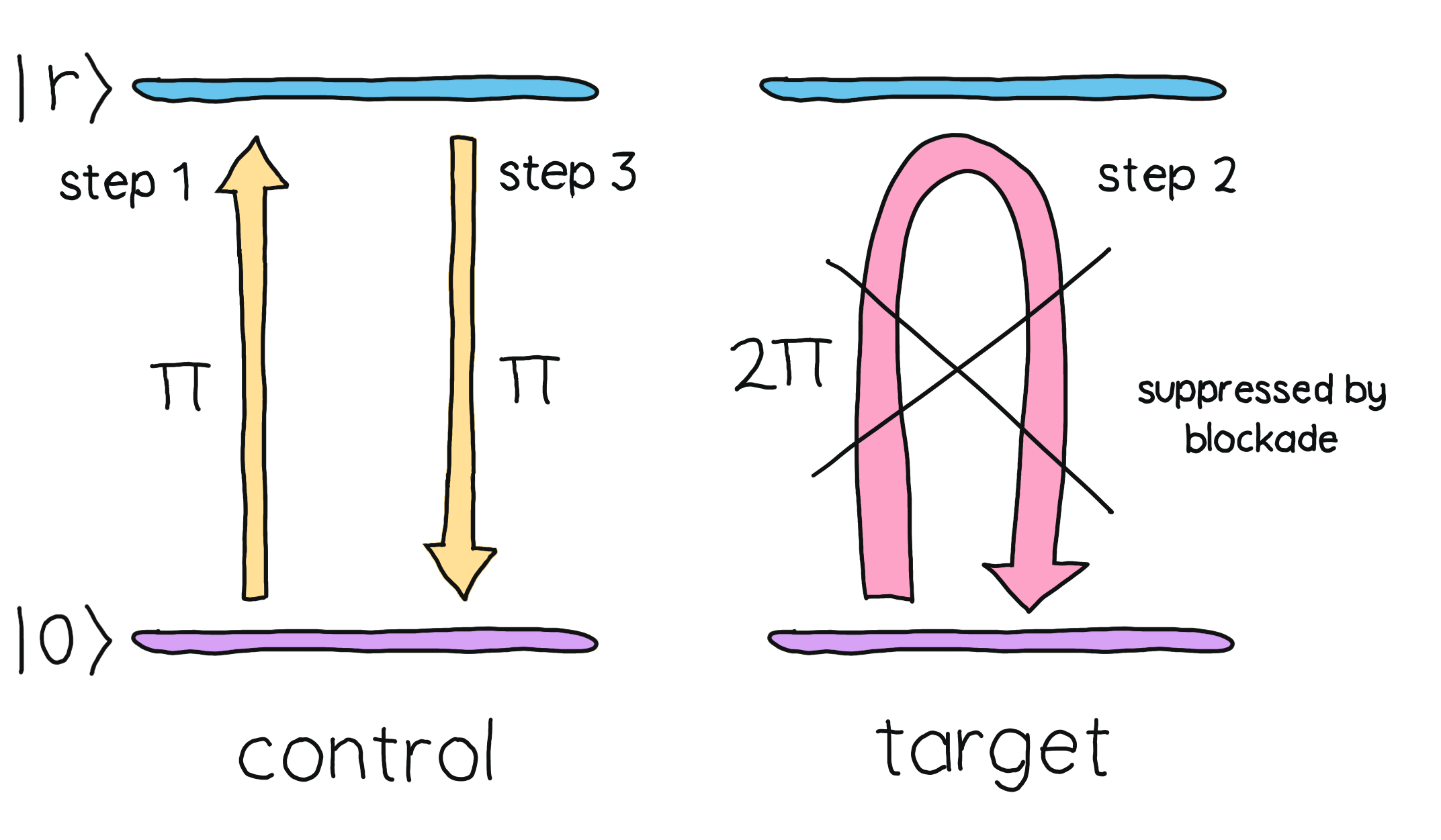
If one of the atoms were to be in the state \(\vert 1 \rangle,\) then the pulse wouldn’t affect such an atom since it’s not tuned to the \(\vert r \rangle \rightarrow \vert 1 \rangle\) transition.

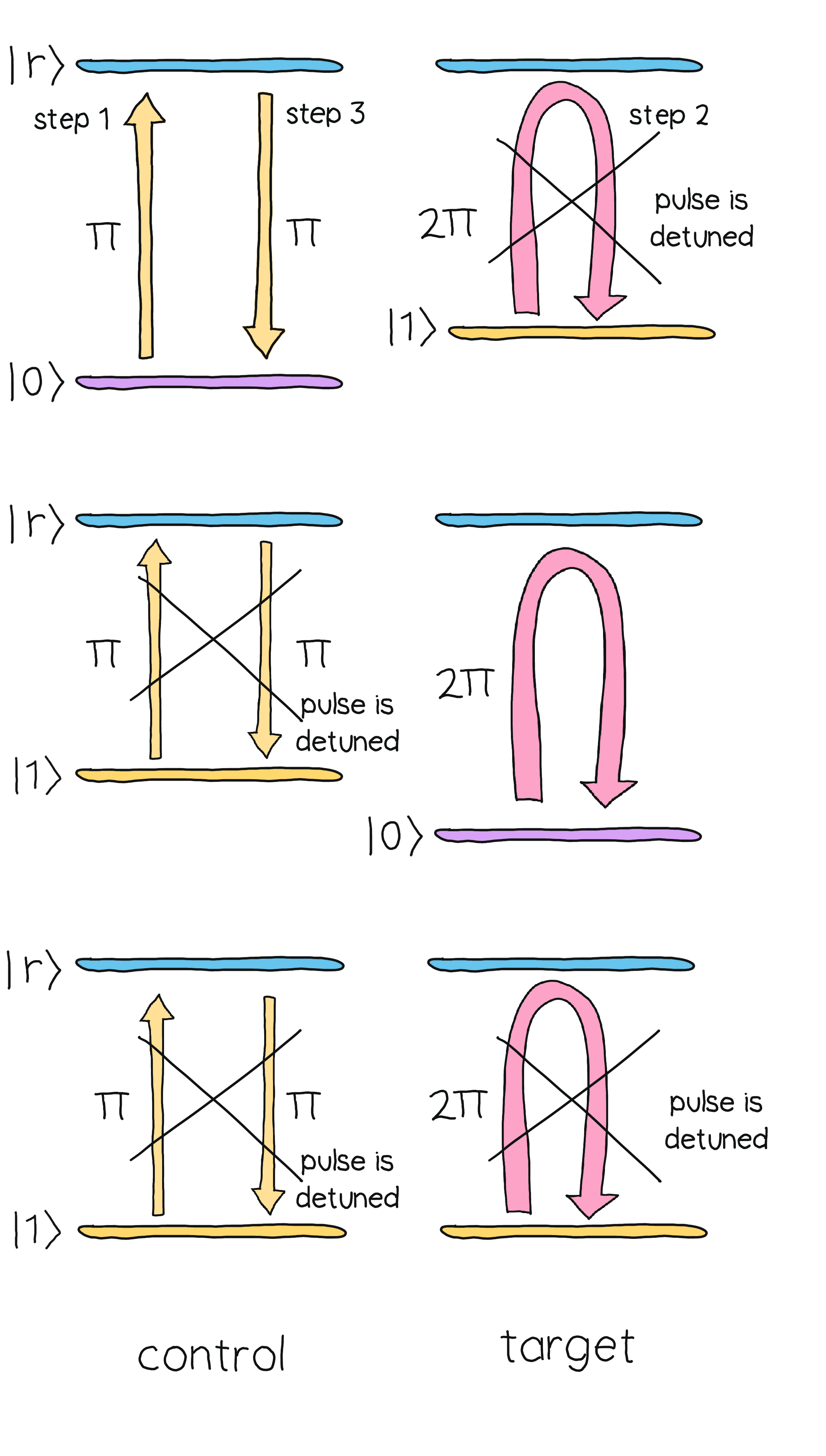
The net effect of the sequence of pulses is summarized in the following table.

Initial state	Final state
\(\vert 00\rangle\)	\(-\vert 00\rangle\)
\(\vert 01\rangle\)	\(-\vert 01\rangle\)
\(\vert 10\rangle\)	\(-\vert 10\rangle\)
\(\vert 11\rangle\)	\(\vert 11\rangle\)

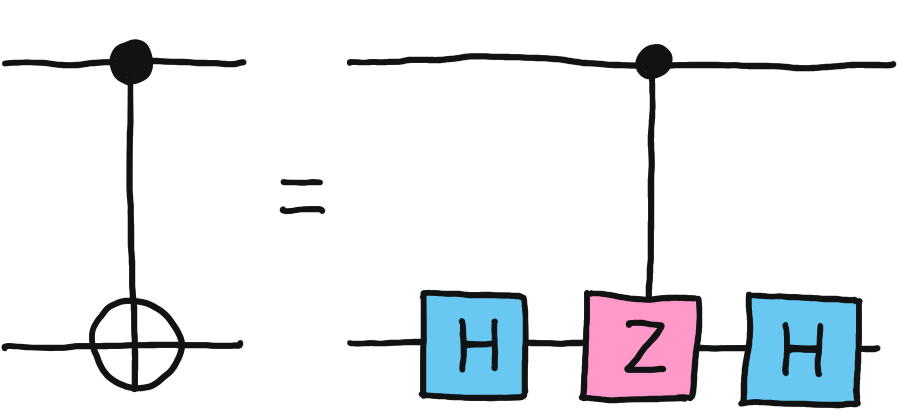
Up to a global phase, this corresponds to the \(CZ\) gate. Together with the \(RX\) and \(RY\) gates, we have a universal set of gates, since the CNOT gate can be expressed in terms of \(CZ\) via the equation

Note

The method shown here is only one of the ways to implement the \(CZ\) gate. Here, we have chosen to encode the qubits in a ground and a hyperfine state, which allows for simplicity. Depending on the hardware, one may also choose to encode the qubits in a ground state and a Rydberg state, or two Rydberg states. The Rydberg blockade is also the main phenomenon that allows for the implementation of two-qubit gates in these realizations, but the details are a bit different 7.

Challenges and future improvements

Great, this all seems to work like a charm… at least in theory. In practice, there are still challenges to overcome. We’ve managed to efficiently prepare qubits, apply gates, and measure, satisfying DiVincenzo’s second, fourth, and fifth criteria. However, as with most quantum architectures, there are some challenges to overcome with regard to scalability and decoherence times.

An important issue to deal with in quantum hardware in general. Quantum states are short-lived in the presence of external influences. We can never achieve a perfect vacuum in the chamber, and the particles and charges around the atoms will destroy our carefully crafted quantum states in a matter of microseconds. While our qubit states are long-lived, the auxiliary Rydberg state is more prone to decohere, which limits the amount of computations we can perform in a succession. Overall improving our register preparation, gates, and measurement protocols is of the essence to make more progress on neutral-atom technology.

While we are able to trap many atoms with our current laser technology, scaling optical tweezer arrays to thousands of qubits poses an obstacle. We rely on spatial modulators to divide our laser beams, but this also reduces the strength of the tweezers. If we split a laser beam too much, the tweezers become too weak to contain an atom. Of course, we could simply use more laser sources, but the spatial requirements for the hardware would also grow. Alternatively, we can use laser sources with higher intensity, but such technology is still being developed. Another solution is to use photons through optical fibres to communicate between different processors, allowing for further connectivity and scalability.

Another issue with scalability is the preparation times of the registers. While, with hundreds of qubits, we can still prepare and arrange the atoms in reasonable times, it becomes increasingly costly the more atoms we have. And we do need to reprepare the neutral atom array when we are done with a computation. It’s not as easy as moving the atoms around faster—if we try to move the atoms around too fast, they will escape from the traps! Therefore, engineers are working on more efficient ways to move the tweezers around, minimizing the number of steps needed to prepare the initial state 8.

Finally, let us remark that there are some nuances with gate implementation—it’s not nearly as simple in real-life as it is in theory. It is not easy to address individual atoms with the driving laser pulses. This is necessary for universal quantum computing, as we saw in the previous section. True local atom drives are still in the works, but even without them, we can still use these non-universal devices for applications in quantum simulation.

Conclusion

Neutral-atom quantum hardware is a promising and quickly developing technology which we should keep an eye on. The ability to easily create custom qubit topologies and the coherence time of the atoms are its main strong points, and its weaknesses are actually no too different from other qubit-based architectures. We can easily program neutral-atom devices using pulses, for which PennyLane is of great help. If you want to learn more, check out our tutorials on the Aquila device, neutral atom configurations, and pulse programming. And do take a look at the references below to dive into much more detail about the topics introduced here.

References

1

QuEra (May 23, 2023). Aquila, our 256-qubit quantum processor, https://www.quera.com/aquila.

2

D. DiVincenzo. (2000) “The Physical Implementation of Quantum Computation”, Fortschritte der Physik 48 (9–11): 771–783. (arXiv)

3

A. Ashkin, J. M. Dziedzic, J. E. Bjorkholm, and Steven Chu. (1986) “Observation of a single-beam gradient force optical trap for dielectric particles”, Opt. Lett. 11, 288-290

4

Atom Computing (May 23, 2023). Quantum Computing Technology, https://atom-computing.com/quantum-computing-technology.

5(1,2)

L. Henriet, et al. (2020) “Quantum computing with neutral atoms”, Quantum volume 4, pg. 327 (arXiv).

6

H. Silverio et al. (2022) “Pulser: An open-source package for the design of pulse sequences in programmable neutral-atom arrays”, Quantum volume 6, pg. 629 (arXiv).

7

M. Morgado and S. Whitlock.(2021) “Quantum simulation and computing with Rydberg-interacting qubits” AVS Quantum Sci. 3, 023501 (arXiv).

8

K. Wintersperger et al. (2023) “Neutral Atom Quantum Computing Hardware: Performance and End-User Perspective”, (arXiv)

About the author

Alvaro Ballon

Alvaro is a quantum computing educator at Xanadu. His work involves making the latest developments in quantum computing accessible to the community.

demos/tutorial_neutral_atoms

 

Download Python script

 

Download Notebook

 

View on GitHub