Machine learning for quantum many-body problems

Author: Utkarsh Azad — Posted: 02 May 2022. Last Updated: 09 May 2022

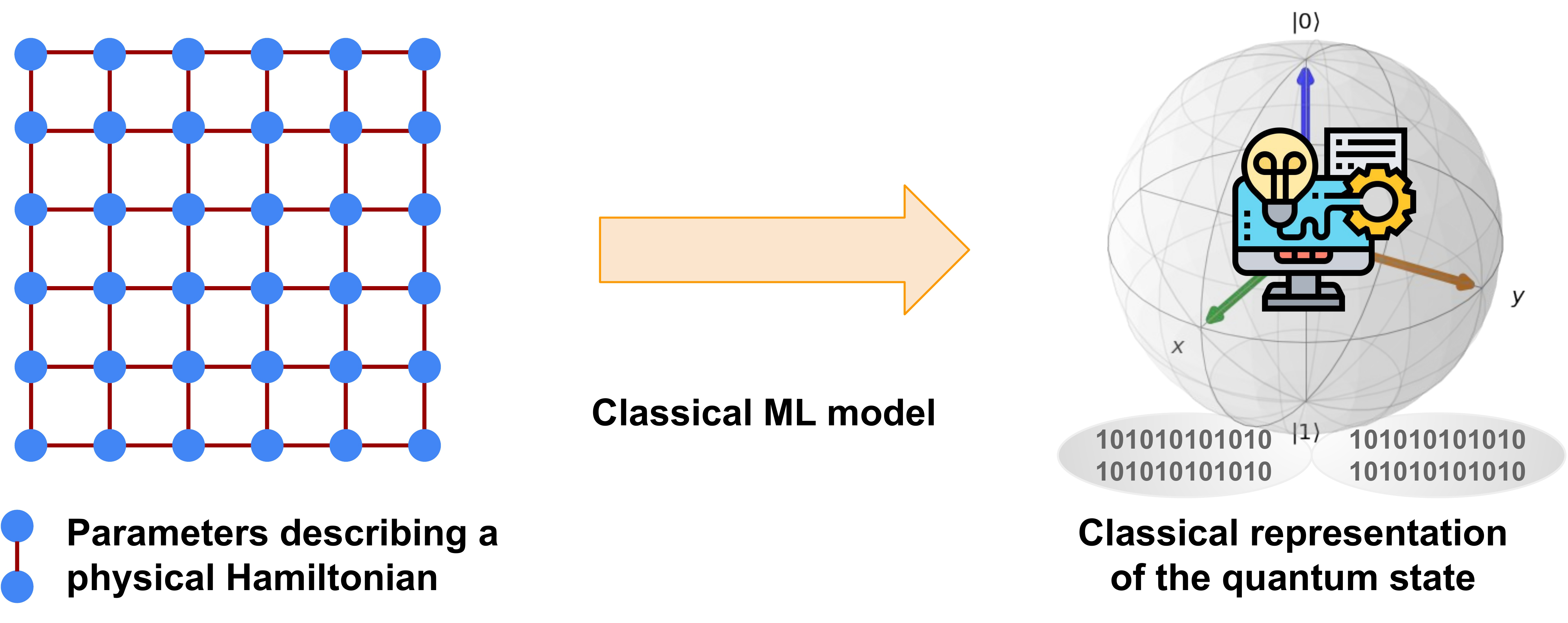
Storing and processing a complete description of an \(n\)-qubit quantum mechanical system is challenging because the amount of memory required generally scales exponentially with the number of qubits. The quantum community has recently addressed this challenge by using the classical shadow formalism, which allows us to build more concise classical descriptions of quantum states using randomized single-qubit measurements. It was argued in Ref. 1 that combining classical shadows with classical machine learning enables using learning models that efficiently predict properties of the quantum systems, such as the expectation value of a Hamiltonian, correlation functions, and entanglement entropies.

Combining machine learning and classical shadows

In this demo, we describe one of the ideas presented in Ref. 1 for using classical shadow formalism and machine learning to predict the ground-state properties of the 2D antiferromagnetic Heisenberg model. We begin by learning how to build the Heisenberg model, calculate its ground-state properties, and compute its classical shadow. Finally, we demonstrate how to use kernel-based learning models to predict ground-state properties from the learned classical shadows. So let’s get started!

Building the 2D Heisenberg Model

We define a two-dimensional antiferromagnetic Heisenberg model as a square lattice, where a spin-1/2 particle occupies each site. The antiferromagnetic nature and the overall physics of this model depend on the couplings \(J_{ij}\) present between the spins, as reflected in the Hamiltonian associated with the model:

\[H = \sum_{i < j} J_{ij}(X_i X_j + Y_i Y_j + Z_i Z_j) .\]

Here, we consider the family of Hamiltonians where all the couplings \(J_{ij}\) are sampled uniformly from [0, 2]. We build a coupling matrix \(J\) by providing the number of rows \(N_r\) and columns \(N_c\) present in the square lattice. The dimensions of this matrix are \(N_s \times N_s\), where \(N_s = N_r \times N_c\) is the total number of spin particles present in the model.

import itertools as it
import pennylane.numpy as np
import numpy as anp

def build_coupling_mats(num_mats, num_rows, num_cols):
    num_spins = num_rows * num_cols
    coupling_mats = np.zeros((num_mats, num_spins, num_spins))
    coup_terms = anp.random.RandomState(24).uniform(0, 2,
                        size=(num_mats, 2 * num_rows * num_cols - num_rows - num_cols))
    # populate edges to build the grid lattice
    edges = [(si, sj) for (si, sj) in it.combinations(range(num_spins), 2)
                        if sj % num_cols and sj - si == 1 or sj - si == num_cols]
    for itr in range(num_mats):
        for ((i, j), term) in zip(edges, coup_terms[itr]):
            coupling_mats[itr][i][j] = coupling_mats[itr][j][i] = term
    return coupling_mats

For this demo, we study a model with four spins arranged on the nodes of a square lattice. We require four qubits for simulating this model; one qubit for each spin. We start by building a coupling matrix J_mat using our previously defined function.

Nr, Nc = 2, 2
num_qubits = Nr * Nc  # Ns
J_mat = build_coupling_mats(1, Nr, Nc)[0]

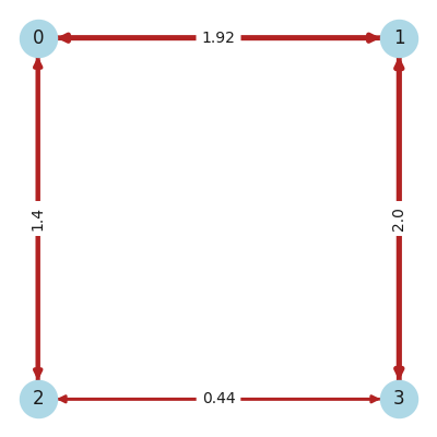
We can now visualize the model instance by representing the coupling matrix as a networkx graph:

import matplotlib.pyplot as plt
import networkx as nx

G = nx.from_numpy_matrix(np.matrix(J_mat), create_using=nx.DiGraph)
pos = {i: (i % Nc, -(i // Nc)) for i in G.nodes()}
edge_labels = {(x, y): np.round(J_mat[x, y], 2) for x, y in G.edges()}
weights = [x + 1.5 for x in list(nx.get_edge_attributes(G, "weight").values())]

plt.figure(figsize=(4, 4))
nx.draw(
    G, pos, node_color="lightblue", with_labels=True,
    node_size=600, width=weights, edge_color="firebrick",
)
nx.draw_networkx_edge_labels(G, pos=pos, edge_labels=edge_labels)
plt.show()

We then use the same coupling matrix J_mat to obtain the Hamiltonian \(H\) for the model we have instantiated above.

import pennylane as qml

def Hamiltonian(J_mat):
    coeffs, ops = [], []
    ns = J_mat.shape[0]
    for i, j in it.combinations(range(ns), r=2):
        coeff = J_mat[i, j]
        if coeff:
            for op in [qml.PauliX, qml.PauliY, qml.PauliZ]:
                coeffs.append(coeff)
                ops.append(op(i) @ op(j))
    H = qml.Hamiltonian(coeffs, ops)
    return H

print(f"Hamiltonian =\n{Hamiltonian(J_mat)}")

Out:

Hamiltonian =
  (0.44013459956570355) [X2 X3]
+ (0.44013459956570355) [Y2 Y3]
+ (0.44013459956570355) [Z2 Z3]
+ (1.399024099899152) [X0 X2]
+ (1.399024099899152) [Y0 Y2]
+ (1.399024099899152) [Z0 Z2]
+ (1.920034606671837) [X0 X1]
+ (1.920034606671837) [Y0 Y1]
+ (1.920034606671837) [Z0 Z1]
+ (1.9997345852477584) [X1 X3]
+ (1.9997345852477584) [Y1 Y3]
+ (1.9997345852477584) [Z1 Z3]

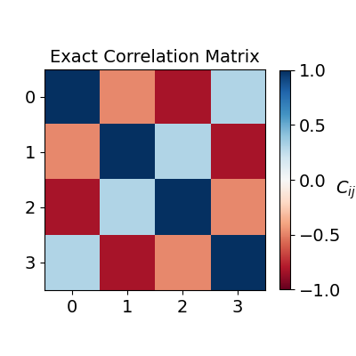
For the Heisenberg model, a property of interest is usually the two-body correlation function \(C_{ij}\), which for a pair of spins \(i\) and \(j\) is defined as the following operator:

\[\hat{C}_{ij} = \frac{1}{3} (X_i X_j + Y_iY_j + Z_iZ_j).\]

def corr_function(i, j):
    ops = []
    for op in [qml.PauliX, qml.PauliY, qml.PauliZ]:
        if i != j:
            ops.append(op(i) @ op(j))
        else:
            ops.append(qml.Identity(i))
    return ops

The expectation value of each such operator \(\hat{C}_{ij}\) with respect to the ground state \(|\psi_{0}\rangle\) of the model can be used to build the correlation matrix \(C\):

\[{C}_{ij} = \langle \hat{C}_{ij} \rangle = \frac{1}{3} \langle \psi_{0} | X_i X_j + Y_iY_j + Z_iZ_j | \psi_{0} \rangle .\]

Hence, to build \(C\) for the model, we need to calculate its ground state \(|\psi_{0}\rangle\). We do this by diagonalizing the Hamiltonian for the model. Then, we obtain the eigenvector corresponding to the smallest eigenvalue.

import scipy as sp

ham = Hamiltonian(J_mat)
eigvals, eigvecs = sp.sparse.linalg.eigs(ham.sparse_matrix())
psi0 = eigvecs[:, np.argmin(eigvals)]

We then build a circuit that initializes the qubits into the ground state and measures the expectation value of the provided set of observables.

dev_exact = qml.device("default.qubit", wires=num_qubits) # for exact simulation

def circuit(psi, observables):
    psi = psi / np.linalg.norm(psi) # normalize the state
    qml.QubitStateVector(psi, wires=range(num_qubits))
    return [qml.expval(o) for o in observables]

circuit_exact = qml.QNode(circuit, dev_exact)

Finally, we execute this circuit to obtain the exact correlation matrix \(C\). We compute the correlation operators \(\hat{C}_{ij}\) and their expectation values with respect to the ground state \(|\psi_0\rangle\).

coups = list(it.product(range(num_qubits), repeat=2))
corrs = [corr_function(i, j) for i, j in coups]

def build_exact_corrmat(coups, corrs, circuit, psi):
    corr_mat_exact = np.zeros((num_qubits, num_qubits))
    for idx, (i, j) in enumerate(coups):
        corr = corrs[idx]
        if i == j:
            corr_mat_exact[i][j] = 1.0
        else:
            corr_mat_exact[i][j] = (
                np.sum(np.array([circuit(psi, observables=[o]) for o in corr]).T) / 3
            )
            corr_mat_exact[j][i] = corr_mat_exact[i][j]
    return corr_mat_exact

expval_exact = build_exact_corrmat(coups, corrs, circuit_exact, psi0)

Once built, we can visualize the correlation matrix:

fig, ax = plt.subplots(1, 1, figsize=(4, 4))
im = ax.imshow(expval_exact, cmap=plt.get_cmap("RdBu"), vmin=-1, vmax=1)
ax.xaxis.set_ticks(range(num_qubits))
ax.yaxis.set_ticks(range(num_qubits))
ax.xaxis.set_tick_params(labelsize=14)
ax.yaxis.set_tick_params(labelsize=14)
ax.set_title("Exact Correlation Matrix", fontsize=14)

bar = fig.colorbar(im, pad=0.05, shrink=0.80    )
bar.set_label(r"$C_{ij}$", fontsize=14, rotation=0)
bar.ax.tick_params(labelsize=14)
plt.show()

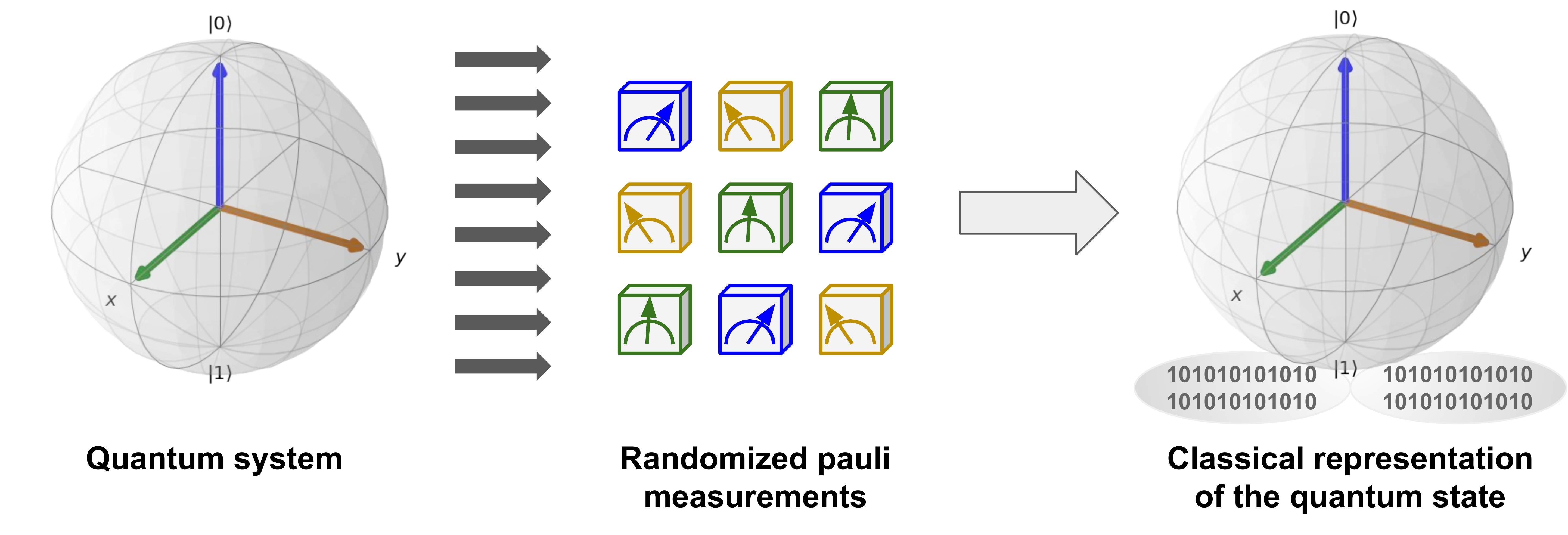
Constructing Classical Shadows

Now that we have built the Heisenberg model, the next step is to construct a classical shadow representation for its ground state. To construct an approximate classical representation of an \(n\)-qubit quantum state \(\rho\), we perform randomized single-qubit measurements on \(T\)-copies of \(\rho\). Each measurement is chosen randomly among the Pauli bases \(X\), \(Y\), or \(Z\) to yield random \(n\) pure product states \(|s_i\rangle\) for each copy:

\[|s_{i}^{(t)}\rangle \in \{|0\rangle, |1\rangle, |+\rangle, |-\rangle, |i+\rangle, |i-\rangle\}.\]

\[S_T(\rho) = \big\{|s_{i}^{(t)}\rangle: i\in\{1,\ldots, n\},\ t\in\{1,\ldots, T\} \big\}.\]

Each of the \(|s_i^{(t)}\rangle\) provides us with a snapshot of the state \(\rho\), and the \(nT\) measurements yield the complete set \(S_{T}\), which requires just \(3nT\) bits to be stored in classical memory. This is discussed in further detail in our previous demo about classical shadows.

To prepare a classical shadow for the ground state of the Heisenberg model, we simply reuse the circuit template used above and reconstruct a QNode utilizing a device that performs single-shot measurements.

dev_oshot = qml.device("default.qubit", wires=num_qubits, shots=1)
circuit_oshot = qml.QNode(circuit, dev_oshot)

Now, we define a function to build the classical shadow for the quantum state prepared by a given \(n\)-qubit circuit using \(T\)-copies of randomized Pauli basis measurements

def gen_class_shadow(circ_template, circuit_params, num_shadows, num_qubits):
    # prepare the complete set of available Pauli operators
    unitary_ops = [qml.PauliX, qml.PauliY, qml.PauliZ]
    # sample random Pauli measurements uniformly
    unitary_ensmb = np.random.randint(0, 3, size=(num_shadows, num_qubits), dtype=int)

    outcomes = np.zeros((num_shadows, num_qubits))
    for ns in range(num_shadows):
        # for each snapshot, extract the Pauli basis measurement to be performed
        meas_obs = [unitary_ops[unitary_ensmb[ns, i]](i) for i in range(num_qubits)]
        # perform single shot randomized Pauli measuremnt for each qubit
        outcomes[ns, :] = circ_template(circuit_params, observables=meas_obs)

    return outcomes, unitary_ensmb


outcomes, basis = gen_class_shadow(circuit_oshot, psi0, 100, num_qubits)
print("First five measurement outcomes =\n", outcomes[:5])
print("First five measurement bases =\n", basis[:5])

Out:

First five measurement outcomes =
 [[ 1. -1. -1. -1.]
 [-1.  1.  1. -1.]
 [ 1.  1. -1. -1.]
 [ 1.  1. -1.  1.]
 [ 1. -1.  1.  1.]]
First five measurement bases =
 [[1 2 2 0]
 [0 0 0 1]
 [1 2 1 2]
 [0 2 2 1]
 [2 0 0 0]]

Furthermore, \(S_{T}\) can be used to construct an approximation of the underlying \(n\)-qubit state \(\rho\) by averaging over \(\sigma_t\):

\[\sigma_T(\rho) = \frac{1}{T} \sum_{1}^{T} \big(3|s_{1}^{(t)}\rangle\langle s_1^{(t)}| - \mathbb{I}\big)\otimes \ldots \otimes \big(3|s_{n}^{(t)}\rangle\langle s_n^{(t)}| - \mathbb{I}\big).\]

def snapshot_state(meas_list, obs_list):
    # undo the rotations done for performing Pauli measurements in the specific basis
    rotations = [
        qml.matrix(qml.Hadamard(wires=0)), # X-basis
        qml.matrix(qml.Hadamard(wires=0)) @ qml.matrix(qml.adjoint(qml.S(wires=0))), # Y-basis
        qml.matrix(qml.Identity(wires=0)), # Z-basis
    ]

    # reconstruct snapshot from local Pauli measurements
    rho_snapshot = [1]
    for meas_out, basis in zip(meas_list, obs_list):
        # preparing state |s_i><s_i| using the post measurement outcome:
        # |0><0| for 1 and |1><1| for -1
        state = np.array([[1, 0], [0, 0]]) if meas_out == 1 else np.array([[0, 0], [0, 1]])
        local_rho = 3 * (rotations[basis].conj().T @ state @ rotations[basis]) - np.eye(2)
        rho_snapshot = np.kron(rho_snapshot, local_rho)

    return rho_snapshot

def shadow_state_reconst(shadow):
    num_snapshots, num_qubits = shadow[0].shape
    meas_lists, obs_lists = shadow

    # Reconstruct the quantum state from its classical shadow
    shadow_rho = np.zeros((2 ** num_qubits, 2 ** num_qubits), dtype=complex)
    for i in range(num_snapshots):
        shadow_rho += snapshot_state(meas_lists[i], obs_lists[i])

    return shadow_rho / num_snapshots

To see how well the reconstruction works for different values of \(T\), we look at the fidelity of the actual quantum state with respect to the reconstructed quantum state from the classical shadow with \(T\) copies. On average, as the number of copies \(T\) is increased, the reconstruction becomes more effective with average higher fidelity values (orange) and lower variance (blue). Eventually, in the limit \(T\rightarrow\infty\), the reconstruction will be exact.

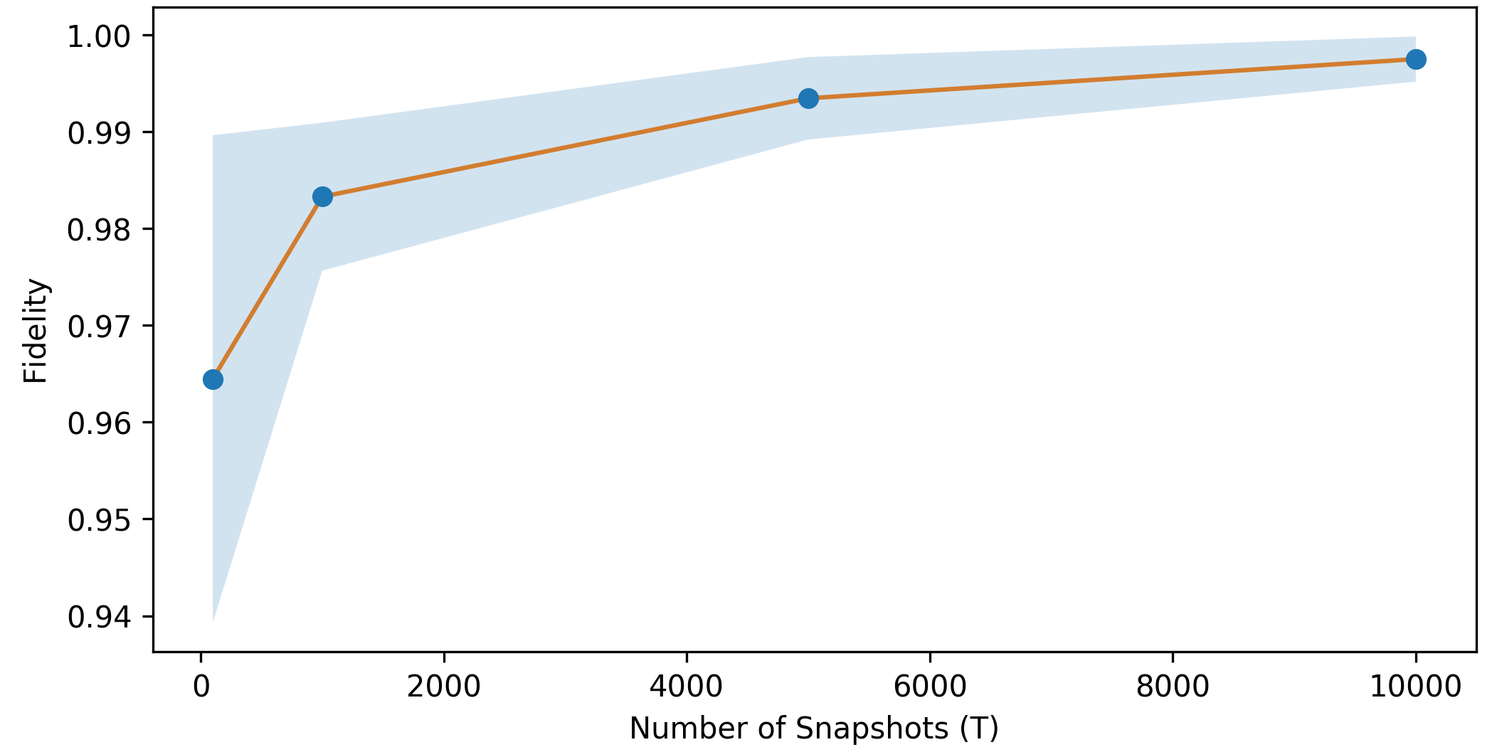
Fidelity of the reconstructed ground state with different shadow sizes \(T\)

The reconstructed quantum state \(\sigma_T\) can also be used to evaluate expectation values \(\text{Tr}(O\sigma_T)\) for some localized observable \(O = \bigotimes_{i}^{n} P_i\), where \(P_i \in \{I, X, Y, Z\}\). However, as shown above, \(\sigma_T\) would be only an approximation of \(\rho\) for finite values of \(T\). Therefore, to estimate \(\langle O \rangle\) robustly, we use the median of means estimation. For this purpose, we split up the \(T\) shadows into \(K\) equally-sized groups and evaluate the median of the mean value of \(\langle O \rangle\) for each of these groups.

def estimate_shadow_obs(shadow, observable, k=10):
    shadow_size = shadow[0].shape[0]

    # convert Pennylane observables to indices
    map_name_to_int = {"PauliX": 0, "PauliY": 1, "PauliZ": 2}
    if isinstance(observable, (qml.PauliX, qml.PauliY, qml.PauliZ)):
        target_obs = np.array([map_name_to_int[observable.name]])
        target_locs = np.array([observable.wires[0]])
    else:
        target_obs = np.array([map_name_to_int[o.name] for o in observable.obs])
        target_locs = np.array([o.wires[0] for o in observable.obs])

    # perform median of means to return the result
    means = []
    meas_list, obs_lists = shadow
    for i in range(0, shadow_size, shadow_size // k):
        meas_list_k, obs_lists_k = (
            meas_list[i : i + shadow_size // k],
            obs_lists[i : i + shadow_size // k],
        )
        indices = np.all(obs_lists_k[:, target_locs] == target_obs, axis=1)
        if sum(indices):
            means.append(
                np.sum(np.prod(meas_list_k[indices][:, target_locs], axis=1)) / sum(indices)
            )
        else:
            means.append(0)

    return np.median(means)

Now we estimate the correlation matrix \(C^{\prime}\) from the classical shadow approximation of the ground state.

coups = list(it.product(range(num_qubits), repeat=2))
corrs = [corr_function(i, j) for i, j in coups]
qbobs = [qob for qobs in corrs for qob in qobs]

def build_estim_corrmat(coups, corrs, num_obs, shadow):
    k = int(2 * np.log(2 * num_obs)) # group size
    corr_mat_estim = np.zeros((num_qubits, num_qubits))
    for idx, (i, j) in enumerate(coups):
        corr = corrs[idx]
        if i == j:
            corr_mat_estim[i][j] = 1.0
        else:
            corr_mat_estim[i][j] = (
                np.sum(np.array([estimate_shadow_obs(shadow, o, k=k+1) for o in corr])) / 3
            )
            corr_mat_estim[j][i] = corr_mat_estim[i][j]
    return corr_mat_estim

shadow = gen_class_shadow(circuit_oshot, psi0, 1000, num_qubits)
expval_estmt = build_estim_corrmat(coups, corrs, len(qbobs), shadow)

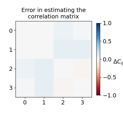
This time, let us visualize the deviation observed between the exact correlation matrix (\(C\)) and the estimated correlation matrix (\(C^{\prime}\)) to assess the effectiveness of classical shadow formalism.

fig, ax = plt.subplots(1, 1, figsize=(4.2, 4))
im = ax.imshow(expval_exact-expval_estmt, cmap=plt.get_cmap("RdBu"), vmin=-1, vmax=1)
ax.xaxis.set_ticks(range(num_qubits))
ax.yaxis.set_ticks(range(num_qubits))
ax.xaxis.set_tick_params(labelsize=14)
ax.yaxis.set_tick_params(labelsize=14)
ax.set_title("Error in estimating the\ncorrelation matrix", fontsize=14)

bar = fig.colorbar(im, pad=0.05, shrink=0.80)
bar.set_label(r"$\Delta C_{ij}$", fontsize=14, rotation=0)
bar.ax.tick_params(labelsize=14)
plt.show()

Training Classical Machine Learning Models

There are multiple ways in which we can combine classical shadows and machine learning. This could include training a model to learn the classical representation of quantum systems based on some system parameter, estimating a property from such learned classical representations, or a combination of both. In our case, we consider the problem of using kernel-based models to learn the ground-state representation of the Heisenberg model Hamiltonian \(H(x_l)\) from the coupling vector \(x_l\), where \(x_l = [J_{i,j} \text{ for } i < j]\). The goal is to predict the correlation functions \(C_{ij}\):

\[\big\{x_l \rightarrow \sigma_T(\rho(x_l)) \rightarrow \text{Tr}(\hat{C}_{ij} \sigma_T(\rho(x_l))) \big\}_{l=1}^{N}.\]

Here, we consider the following kernel-based machine learning model 2:

\[\hat{\sigma}_{N} (x) = \sum_{l=1}^{N} \kappa(x, x_l)\sigma_T (x_l) = \sum_{l=1}^{N} \left(\sum_{l^{\prime}=1}^{N} k(x, x_{l^{\prime}})(K+\lambda I)^{-1}_{l, l^{\prime}} \sigma_T(x_l) \right),\]

where \(\lambda > 0\) is a regularization parameter in cases when \(K\) is not invertible, \(\sigma_T(x_l)\) denotes the classical representation of the ground state \(\rho(x_l)\) of the Heisenberg model constructed using \(T\) randomized Pauli measurements, and \(K_{ij}=k(x_i, x_j)\) is the kernel matrix with \(k(x, x^{\prime})\) as the kernel function.

Similarly, estimating an expectation value on the predicted ground state \(\sigma_T(x_l)\) using the trained model can then be done by evaluating:

\[\text{Tr}(\hat{O} \hat{\sigma}_{N} (x)) = \sum_{l=1}^{N} \kappa(x, x_l)\text{Tr}(O\sigma_T (x_l)).\]

We train the classical kernel-based models using \(N = 70\) randomly chosen values of the coupling matrices \(J\).

# imports for ML methods and techniques
from sklearn.model_selection import train_test_split, cross_val_score
from sklearn import svm
from sklearn.kernel_ridge import KernelRidge

First, to build the dataset, we use the function build_dataset that takes as input the size of the dataset (num_points), the topology of the lattice (Nr and Nc), and the number of randomized Pauli measurements (\(T\)) for the construction of classical shadows. The X_data is the set of coupling vectors that are defined as a stripped version of the coupling matrix \(J\), where only non-duplicate and non-zero \(J_{ij}\) are considered. The y_exact and y_clean are the set of correlation vectors, i.e., the flattened correlation matrix \(C\), computed with respect to the ground-state obtained from exact diagonalization and classical shadow representation (with \(T=500\)), respectively.

def build_dataset(num_points, Nr, Nc, T=500):

    num_qubits = Nr * Nc
    X, y_exact, y_estim = [], [], []
    coupling_mats = build_coupling_mats(num_points, Nr, Nc)

    for coupling_mat in coupling_mats:
        ham = Hamiltonian(coupling_mat)
        eigvals, eigvecs = sp.sparse.linalg.eigs(ham.sparse_matrix())
        psi = eigvecs[:, np.argmin(eigvals)]
        shadow = gen_class_shadow(circuit_oshot, psi, T, num_qubits)

        coups = list(it.product(range(num_qubits), repeat=2))
        corrs = [corr_function(i, j) for i, j in coups]
        qbobs = [x for sublist in corrs for x in sublist]

        expval_exact = build_exact_corrmat(coups, corrs, circuit_exact, psi)
        expval_estim = build_estim_corrmat(coups, corrs, len(qbobs), shadow)

        coupling_vec = []
        for coup in coupling_mat.reshape(1, -1)[0]:
            if coup and coup not in coupling_vec:
                coupling_vec.append(coup)
        coupling_vec = np.array(coupling_vec) / np.linalg.norm(coupling_vec)

        X.append(coupling_vec)
        y_exact.append(expval_exact.reshape(1, -1)[0])
        y_estim.append(expval_estim.reshape(1, -1)[0])

    return np.array(X), np.array(y_exact), np.array(y_estim)

X, y_exact, y_estim = build_dataset(100, Nr, Nc, 500)
X_data, y_data = X, y_estim
X_data.shape, y_data.shape, y_exact.shape

Out:

((100, 4), (100, 16), (100, 16))

Now that our dataset is ready, we can shift our focus to the ML models. Here, we use two different Kernel functions: (i) Gaussian Kernel and (ii) Neural Tangent Kernel. For both of them, we consider the regularization parameter \(\lambda\) from the following set of values:

\[\lambda = \left\{ 0.0025, 0.0125, 0.025, 0.05, 0.125, 0.25, 0.5, 1.0, 5.0, 10.0 \right\}.\]

Next, we define the kernel functions \(k(x, x^{\prime})\) for each of the mentioned kernels:

\[k(x, x^{\prime}) = e^{-\gamma||x - x^{\prime}||^{2}_{2}}. \tag{Gaussian Kernel}\]

For the Gaussian kernel, the hyperparameter \(\gamma = N^{2}/\sum_{i=1}^{N} \sum_{j=1}^{N} ||x_i-x_j||^{2}_{2} > 0\) is chosen to be the inverse of the average Euclidean distance \(x_i\) and \(x_j\). The kernel is implemented using the radial-basis function (rbf) kernel in the sklearn library.

\[k(x, x^{\prime}) = k^{\text{NTK}}(x, x^{\prime}). \tag{Neural Tangent Kernel}\]

The neural tangent kernel \(k^{\text{NTK}}\) used here is equivalent to an infinite-width feed-forward neural network with four hidden layers and that uses the rectified linear unit (ReLU) as the activation function. This is implemented using the neural_tangents library.

from neural_tangents import stax
init_fn, apply_fn, kernel_fn = stax.serial(
    stax.Dense(32),
    stax.Relu(),
    stax.Dense(32),
    stax.Relu(),
    stax.Dense(32),
    stax.Relu(),
    stax.Dense(32),
    stax.Relu(),
    stax.Dense(1),
)
kernel_NN = kernel_fn(X_data, X_data, "ntk")

for i in range(len(kernel_NN)):
    for j in range(len(kernel_NN)):
        kernel_NN.at[i, j].set((kernel_NN[i][i] * kernel_NN[j][j]) ** 0.5)

For the above two defined kernel methods, we obtain the best learning model by performing hyperparameter tuning using cross-validation for the prediction task of each \(C_{ij}\). For this purpose, we implement the function fit_predict_data, which takes input as the correlation function index cij, kernel matrix kernel, and internal kernel mapping opt required by the kernel-based regression models from the sklearn library.

from sklearn.metrics import mean_squared_error

def fit_predict_data(cij, kernel, opt="linear"):

    # training data (estimated from measurement data)
    y = np.array([y_estim[i][cij] for i in range(len(X_data))])
    X_train, X_test, y_train, y_test = train_test_split(
        kernel, y, test_size=0.3, random_state=24
    )

    # testing data (exact expectation values)
    y_clean = np.array([y_exact[i][cij] for i in range(len(X_data))])
    _, _, _, y_test_clean = train_test_split(kernel, y_clean, test_size=0.3, random_state=24)

    # hyperparameter tuning with cross validation
    models = [
        # Epsilon-Support Vector Regression
        (lambda Cx: svm.SVR(kernel=opt, C=Cx, epsilon=0.1)),
        # Kernel-Ridge based Regression
        (lambda Cx: KernelRidge(kernel=opt, alpha=1 / (2 * Cx))),
    ]

    # Regularization parameter
    hyperparams = [0.0025, 0.0125, 0.025, 0.05, 0.125, 0.25, 0.5, 1.0, 5.0, 10.0]
    best_pred, best_cv_score, best_test_score = None, np.inf, np.inf
    for model in models:
        for hyperparam in hyperparams:
            cv_score = -np.mean(
                cross_val_score(
                    model(hyperparam), X_train, y_train, cv=5,
                    scoring="neg_root_mean_squared_error",
                )
            )
            if best_cv_score > cv_score:
                best_model = model(hyperparam).fit(X_train, y_train)
                best_pred = best_model.predict(X_test)
                best_cv_score = cv_score
                best_test_score = mean_squared_error(
                    best_model.predict(X_test).ravel(), y_test_clean.ravel(), squared=False
                )

    return (
        best_pred, y_test_clean, np.round(best_cv_score, 5), np.round(best_test_score, 5)
    )

We perform the fitting and prediction for each \(C_{ij}\) and print the output in a tabular format.

kernel_list = ["Gaussian kernel", "Neural Tangent kernel"]
kernel_data = np.zeros((num_qubits ** 2, len(kernel_list), 2))
y_predclean, y_predicts1, y_predicts2 = [], [], []

for cij in range(num_qubits ** 2):
    y_predict, y_clean, cv_score, test_score = fit_predict_data(cij, X_data, opt="rbf")
    y_predclean.append(y_clean)
    kernel_data[cij][0] = (cv_score, test_score)
    y_predicts1.append(y_predict)
    y_predict, y_clean, cv_score, test_score = fit_predict_data(cij, kernel_NN)
    kernel_data[cij][1] = (cv_score, test_score)
    y_predicts2.append(y_predict)

# For each C_ij print (best_cv_score, test_score) pair
row_format = "{:>25}{:>35}{:>35}"
print(row_format.format("Correlation", *kernel_list))
for idx, data in enumerate(kernel_data):
    print(
        row_format.format(
            f"\t C_{idx//num_qubits}{idx%num_qubits} \t| ",
            str(data[0]),
            str(data[1]),
        )
    )

Out:

Correlation                    Gaussian kernel              Neural Tangent kernel
   C_00   |                           [-0.  0.]                          [-0.  0.]
   C_01   |                   [0.07928 0.06935]                  [0.10715 0.07989]
   C_02   |                   [0.10111 0.06816]                  [0.11277 0.09275]
   C_03   |                   [0.11402 0.05578]                  [0.1171  0.06899]
   C_10   |                   [0.07928 0.06935]                  [0.10715 0.07989]
   C_11   |                           [-0.  0.]                          [-0.  0.]
   C_12   |                   [0.11408 0.04673]                  [0.11635 0.06798]
   C_13   |                   [0.10033 0.06599]                  [0.11634 0.08031]
   C_20   |                   [0.10111 0.06816]                  [0.11277 0.09275]
   C_21   |                   [0.11408 0.04673]                  [0.11635 0.06798]
   C_22   |                           [-0.  0.]                          [-0.  0.]
   C_23   |                   [0.10059 0.0647 ]                  [0.12249 0.0715 ]
   C_30   |                   [0.11402 0.05578]                  [0.1171  0.06899]
   C_31   |                   [0.10033 0.06599]                  [0.11634 0.08031]
   C_32   |                   [0.10059 0.0647 ]                  [0.12249 0.0715 ]
   C_33   |                           [-0.  0.]                          [-0.  0.]

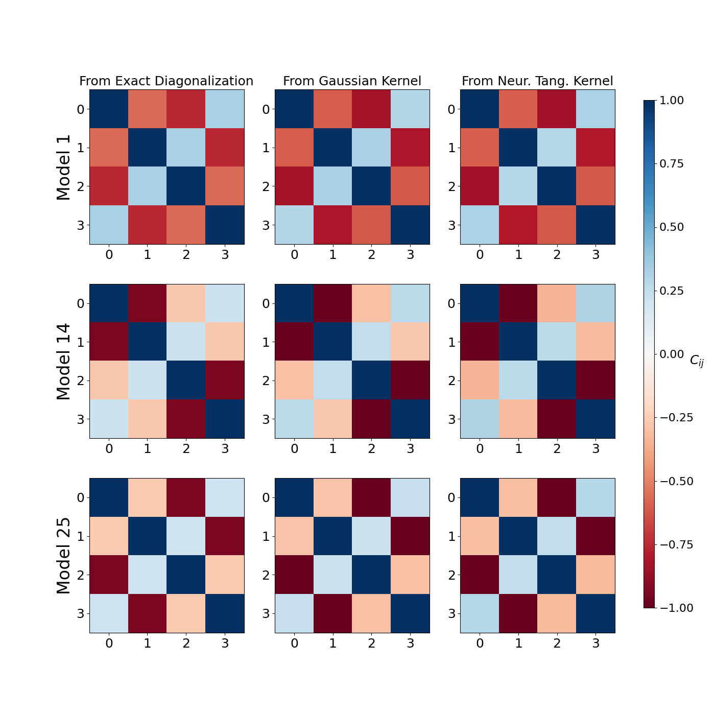
Overall, we find that the models with the Gaussian kernel performed better than those with NTK for predicting the expectation value of the correlation function \(C_{ij}\) for the ground state of the Heisenberg model. However, the best choice of \(\lambda\) differed substantially across the different \(C_{ij}\) for both kernels. We present the predicted correlation matrix \(C^{\prime}\) for randomly selected Heisenberg models from the test set below for comparison against the actual correlation matrix \(C\), which is obtained from the ground state found using exact diagonalization.

fig, axes = plt.subplots(3, 3, figsize=(14, 14))
corr_vals = [y_predclean, y_predicts1, y_predicts2]
plt_plots = [1, 14, 25]

cols = [
    "From {}".format(col)
    for col in ["Exact Diagonalization", "Gaussian Kernel", "Neur. Tang. Kernel"]
]
rows = ["Model {}".format(row) for row in plt_plots]

for ax, col in zip(axes[0], cols):
    ax.set_title(col, fontsize=18)

for ax, row in zip(axes[:, 0], rows):
    ax.set_ylabel(row, rotation=90, fontsize=24)

for itr in range(3):
    for idx, corr_val in enumerate(corr_vals):
        shw = axes[itr][idx].imshow(
            np.array(corr_vals[idx]).T[plt_plots[itr]].reshape(Nr * Nc, Nr * Nc),
            cmap=plt.get_cmap("RdBu"), vmin=-1, vmax=1,
        )
        axes[itr][idx].xaxis.set_ticks(range(Nr * Nc))
        axes[itr][idx].yaxis.set_ticks(range(Nr * Nc))
        axes[itr][idx].xaxis.set_tick_params(labelsize=18)
        axes[itr][idx].yaxis.set_tick_params(labelsize=18)

fig.subplots_adjust(right=0.86)
cbar_ax = fig.add_axes([0.90, 0.15, 0.015, 0.71])
bar = fig.colorbar(shw, cax=cbar_ax)

bar.set_label(r"$C_{ij}$", fontsize=18, rotation=0)
bar.ax.tick_params(labelsize=16)
plt.show()

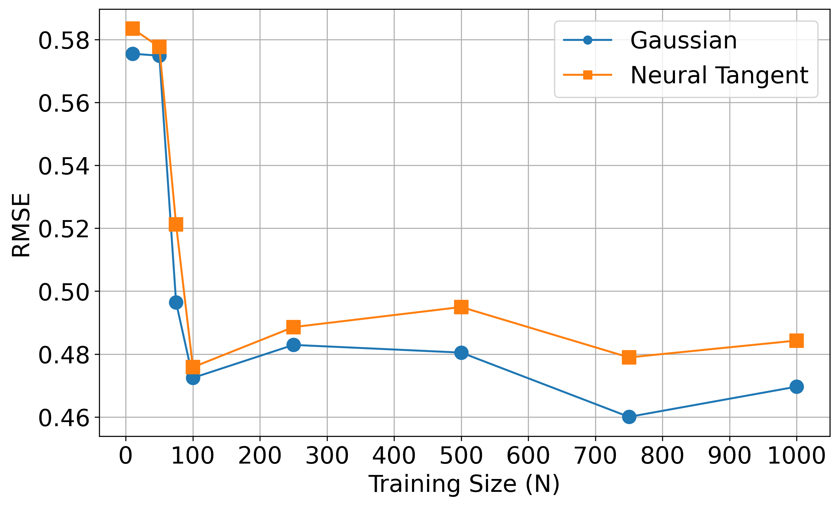
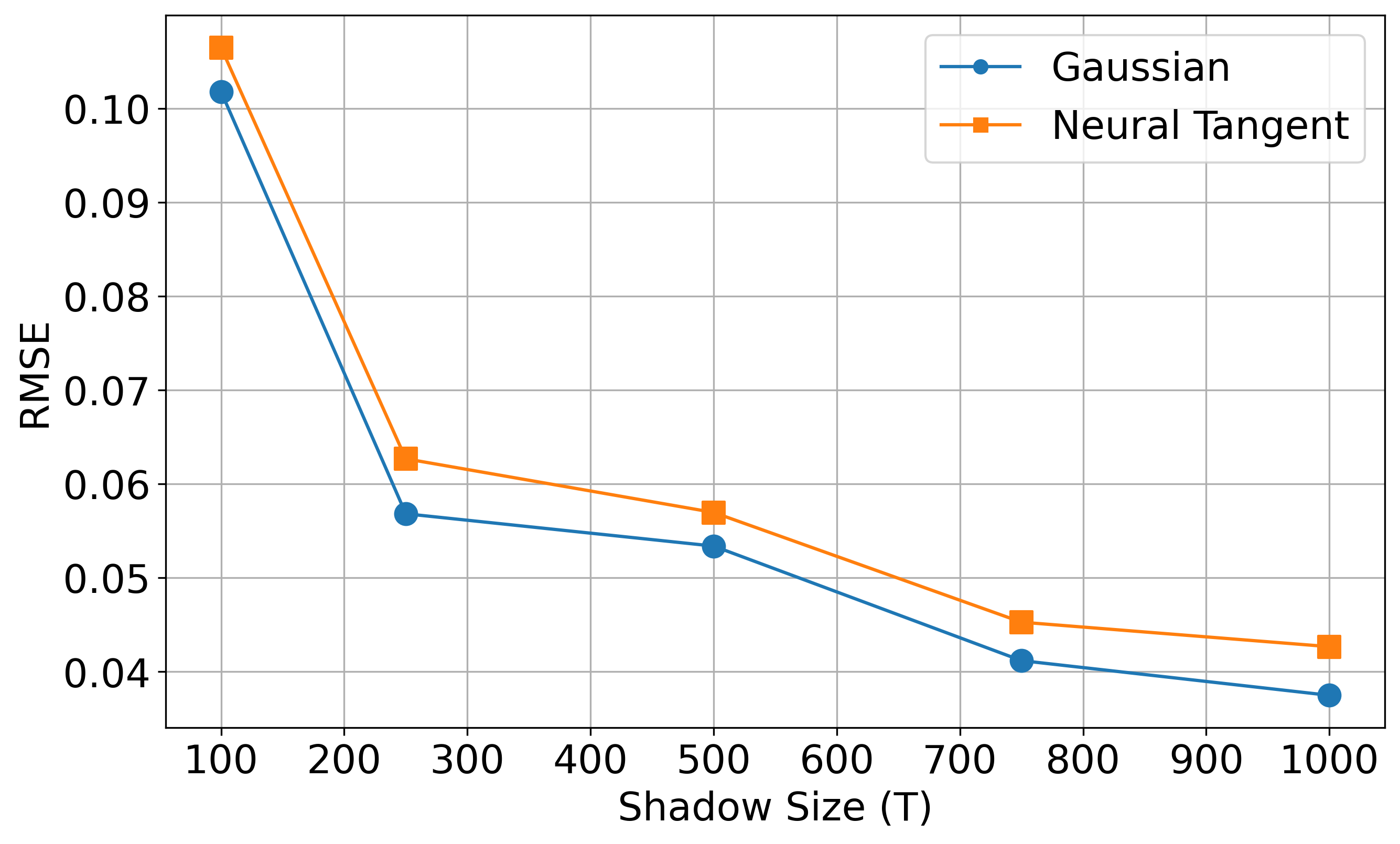
Finally, we also attempt to showcase the effect of the size of training data \(N\) and the number of Pauli measurements \(T\). For this, we look at the average root-mean-square error (RMSE) in prediction for each kernel over all two-point correlation functions \(C_{ij}\). Here, the first plot looks at the different training sizes \(N\) with a fixed number of randomized Pauli measurements \(T=100\). In contrast, the second plot looks at the different shadow sizes \(T\) with a fixed training data size \(N=70\). The performance improvement seems to be saturating after a sufficient increase in \(N\) and \(T\) values for all two kernels in both the cases.

Conclusion

This demo illustrates how classical machine learning models can benefit from the classical shadow formalism for learning characteristics and predicting the behavior of quantum systems. As argued in Ref. 1, this raises the possibility that models trained on experimental or quantum data data can effectively address quantum many-body problems that cannot be solved using classical methods alone.

References

1(1,2,3)

H. Y. Huang, R. Kueng, G. Torlai, V. V. Albert, J. Preskill, “Provably efficient machine learning for quantum many-body problems”, arXiv:2106.12627 [quant-ph] (2021)

2

A. Jacot, F. Gabriel, and C. Hongler. “Neural tangent kernel: Convergence and generalization in neural networks”. NeurIPS, 8571–8580 (2018)

About the author

Utkarsh Azad

Utkarsh is a quantum software researcher at Xanadu, working on making quantum computing more useful and accessible, with a focus on exploring its applications in natural sciences. Whenever he's not tinkering with code, he will be walking miles searching either for fractals in nature or a cup of filter coffee.

demos/tutorial_ml_classical_shadows

 

Download Python script

 

Download Notebook

 

View on GitHub