Quantum advantage with Gaussian Boson Sampling

Authors: Josh Izaac and Nathan Killoran — Posted: 04 December 2020. Last updated: 04 December 2020.

Warning

This demo is only compatible with PennyLane version 0.29 or below.

On the journey to large-scale fault-tolerant quantum computers, one of the first major milestones is to demonstrate a quantum device carrying out tasks that are beyond the reach of any classical algorithm. The launch of Xanadu’s Borealis device marked an important milestone within the quantum computing community, wherein our very own quantum computational advantage experiment using quantum photonics was demonstrated in our Nature paper. Among other quantum advantage achievements are the Google Quantum team’s experiment as can be seen in their paper Quantum supremacy using a programmable superconducting processor 1, and the experiment from the team led by Chao-Yang Lu and Jian-Wei as can be seen in their paper Quantum computational advantage using photons 2.

While Google’s experiment performed the task of random circuit sampling using a superconducting processor, both Chao-Yang Lu and Jian-Wei’s team and Xanadu leveraged the quantum properties of light to tackle a task called Gaussian Boson Sampling (GBS).

This tutorial will walk you through the basic elements of GBS, motivate why it is classically challenging, and show you how to explore GBS using PennyLane and the photonic quantum devices accessible via the PennyLane-Strawberry Fields plugin. If you are interested in possible applications of GBS, or want to access programmable GBS hardware via the cloud, check out the Strawberry Fields website for more details.

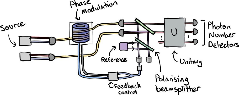
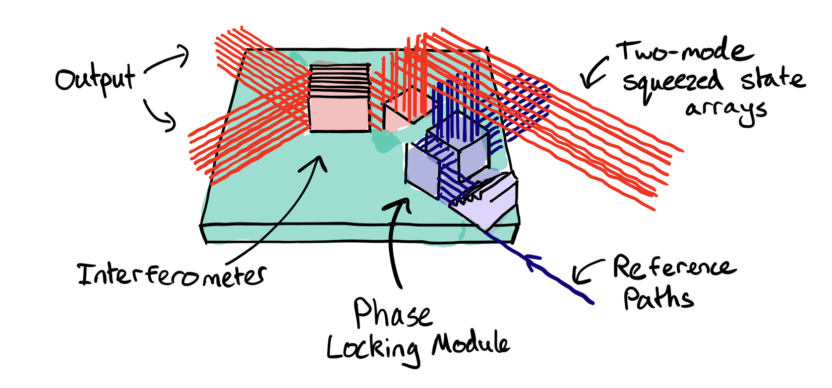
Illustration of the experimental setup used by Zhong et al. in Quantum computational advantage using photons 2.

The origins of GBS

Let’s first explain the name. Boson refers to bosonic matter, which, along with fermions, makes up one of the two elementary classes of particles. The most prevalent bosonic system in our everyday lives is light, which is made of particles called photons. Another famous example, though much harder to find, is the Higgs boson. The distinguishing characteristic of bosons is that they follow “Bose-Einstein statistics”, which very loosely means that the particles like to bunch together (contrast this to fermionic matter like electrons, which must follow the Pauli Exclusion Principle and keep apart).

This property can be observed in simple interference experiments such as the Hong-Ou Mandel setup. If two single photons are interfered on a balanced beamsplitter, they will both emerge at the same output port—there is zero probability that they will emerge at separate outputs. This is a simple but notable quantum property of light; if electrons were brought together in a similar experiement, they would always appear at separate output ports.

Gaussian Boson Sampling 3 is, in fact, a member of a larger family of “Boson Sampling” algorithms, stemming back to the initial proposal of Aaronson and Arkhipov 4 in 2013. Boson Sampling is quantum interferometry writ large. Aaronson and Arkhipov’s original proposal was to inject many single photons into distinct input ports of a large interferometer, then measure which output ports they appear at. The natural interference properties of bosons means that photons will appear at the output ports in very unique and specific ways. Boson Sampling was not proposed with any kind of practical real-world use-case in mind. Like the random circuit sampling, it’s just a quantum system being its best self. With sufficient size and quality, it is strongly believed to be hard for a classical computer to simulate this efficiently.

Finally, the “Gaussian” in GBS refers to the fact that we modify the original Boson Sampling proposal slightly: instead of injecting single photons—which are hard to jointly create in the size and quality needed to demonstrate Boson Sampling conclusively—we instead use states of light that are experimentally less demanding (though still challenging!). These states of light are called Gaussian states, because they bear strong connections to the Gaussian (or Normal) distribution from statistics. In practice, we use a particular Gaussian state called a squeezed state for the inputs, since these are arguably the most non-classical of Gaussian states.

Note

While computationally hard to simulate, Boson Sampling devices, on their own, are not capable of universal quantum computing. However, in combination with other components, GBS is a key building block for a universal device 5.

Coding a GBS algorithm

The researchers in 2 experimentally demonstrate a GBS device by preparing 50 squeezed states and injecting them into a 100-mode interferometer. In this demo, in order to keep things classically simulable, we will stick to a much simpler setting consisting of 4 squeezed states injected into a 4-mode interferometer. At a high level, an interferometer on \(N\) modes can be represented using an \(N\times N\) unitary matrix \(U\). When decomposed into a quantum optical circuit, the interferometer will be made up of beamsplitters and phase shifters.

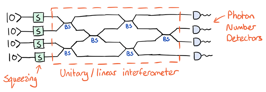
Simulating this circuit using PennyLane is easy; we can simply read off the gates from left to right, and convert it into a QNode.

import numpy as np

# set the random seed
np.random.seed(42)

# import PennyLane
import pennylane as qml

We must define the unitary matrix we would like to embed in the circuit. We will use SciPy to generate a Haar-random unitary:

from scipy.stats import unitary_group

# define the linear interferometer
U = unitary_group.rvs(4)
print(U)

Out:

[[ 0.23648826-0.48221431j  0.06829648+0.04447898j  0.51150074-0.09529866j
  0.55205719-0.35974699j]
 [-0.11148167+0.69780321j -0.24943828+0.08410701j  0.46705929-0.43192981j
   0.16220654-0.01817602j]
[-0.22351926-0.25918352j  0.24364996-0.05375623j -0.09259829-0.53810588j
   0.27267708+0.66941977j]
  [ 0.11519953-0.28596729j -0.90164923-0.22099186j -0.09627758-0.13105595j
  -0.0200152 +0.12766128j]]

We can now use this to construct the circuit, choosing a compatible device. For the simulation, we can use the Strawberry Fields Gaussian backend. This backend is perfectly suited for simulation of GBS, as the initial states are Gaussian, and all gates transform Gaussian states to other Gaussian states.

n_wires = 4
cutoff = 10

dev = qml.device("strawberryfields.gaussian", wires=n_wires, cutoff_dim=cutoff)


@qml.qnode(dev)
def gbs_circuit():
    # prepare the input squeezed states
    for i in range(n_wires):
        qml.Squeezing(1.0, 0.0, wires=i)

    # linear interferometer
    qml.InterferometerUnitary(U, wires=range(n_wires))
    return qml.probs(wires=range(n_wires))

A couple of things to note in this particular example:

1. To prepare the input single mode squeezed vacuum state \(|re^{i\phi}\rangle\), where \(r = 1\) and \(\phi=0\), we apply a squeezing gate (Squeezing) to each of the wires (initially in the vacuum state).

2. Next we apply the linear interferometer to all four wires using Interferometer and the unitary matrix U. This operator decomposes the unitary matrix representing the linear interferometer into single-mode rotation gates (PhaseShift) and two-mode beamsplitters (Beamsplitter). After applying the interferometer, we will denote the output state by \(|\psi'\rangle\).

3. GBS takes place physically in an infinite-dimensional Hilbert space, which is not practical for simulation. We need to set an upper limit on the maximum number of photons we can detect. This is the cutoff value we defined above; we will only be considering detection events containing 0 to 9 photons per mode.

We can now execute the QNode, and extract the resulting probability distribution:

probs = gbs_circuit().reshape([cutoff] * n_wires)
print(probs.shape)

Out:

(10, 10, 10, 10)

0 and wire 3, and 2 photons at wire 1, i.e., the value

\[\text{prob}(1,2,0,1) = \left|\langle{1,2,0,1} \mid \psi'\rangle \right|^2.\]

Let’s extract and view the probabilities of measuring various Fock states.

# Fock states to measure at output
measure_states = [(0, 0, 0, 0), (1, 1, 0, 0), (0, 1, 0, 1), (1, 1, 1, 1), (2, 0, 0, 0)]

# extract the probabilities of calculating several
# different Fock states at the output, and print them out
for i in measure_states:
    print(f"|{''.join(str(j) for j in i)}>: {probs[i]}")

Out:

|0000>: 0.17637844761413496
|1100>: 0.03473293649420282
|0101>: 0.011870900427255589
|1111>: 0.005957399165336106
|2000>: 0.02957384308320549

Hamilton et al. 3 showed that the probability of measuring a final state containing only 0 or 1 photons per mode is given by

\[\left|\langle{n_1,n_2,\dots,n_N}\middle|{\psi'}\rangle\right|^2 = \frac{\left|\text{Haf}[(U(\bigoplus_i\mathrm{tanh}(r_i))U^T)]_{st}\right|^2}{\prod_{i=1}^N \cosh(r_i)}\]

i.e., the sampled single-photon probability distribution is proportional to the hafnian of a submatrix of \(U(\bigoplus_i\mathrm{tanh}(r_i))U^T\).

Note

The hafnian of a matrix is defined by

\[\text{Haf}(A) = \sum_{\sigma \in \text{PMP}_{2N}}\prod_{i=1}^N A_{\sigma(2i-1)\sigma(2i)},\]

where \(\text{PMP}_{2N}\) is the set of all perfect matching permutations of \(2N\) elements. In graph theory, the hafnian calculates the number of perfect matchings in a graph with adjacency matrix \(A\).

Compare this to the permanent, which calculates the number of perfect matchings on a bipartite graph. Notably, the permanent appears in vanilla Boson Sampling in a similar way that the hafnian appears in GBS. The hafnian turns out to be a generalization of the permanent, with the relationship

\[\begin{split}\text{Per(A)} = \text{Haf}\left(\left[\begin{matrix} 0&A\\ A^T&0 \end{matrix}\right]\right).\end{split}\]

As any algorithm that could calculate (or even approximate) the hafnian could also calculate the permanent—a #P-hard problem—it follows that calculating or approximating the hafnian must also be a classically hard problem. This lies behind the classical hardness of GBS.

In this demo, we will use the same squeezing parameter, \(z=r\), for all input states; this allows us to simplify this equation. To start with, the hafnian expression simply becomes \(\text{Haf}[(UU^T\mathrm{tanh}(r))]_{st}\), removing the need for the direct sum.

Thus, we have

\[\left|\left\langle{n_1,n_2,\dots,n_N}\middle|{\psi'}\right\rangle\right|^2 = \frac{\left|\text{Haf}[(UU^T\tanh(r))]_{st}\right|^2}{n_1!n_2!\cdots n_N!\cosh^N(r)}.\]

Now that we have the theoretical formulas, as well as the probabilities from our simulated GBS QNode, we can compare the two and see whether they agree.

In order to calculate the probability of different GBS events classically, we need a method for calculating the hafnian. For this, we will use The Walrus library (which is installed as a dependency of the PennyLane-SF plugin):

from thewalrus import hafnian as haf

Now, for the right-hand side numerator, we first calculate the submatrix \(A = [(UU^T\mathrm{tanh}(r))]_{st}\):

A = np.dot(U, U.T) * np.tanh(1)

In GBS, we determine the submatrix by taking the rows and columns corresponding to the measured Fock state. For example, to calculate the submatrix in the case of the output measurement \(\left|{1,1,0,0}\right\rangle\), we have

print(A[:, [0, 1]][[0, 1]])

Out:

[[ 0.19343159-0.54582922j  0.43418269-0.09169615j]
 [ 0.43418269-0.09169615j -0.27554025-0.46222197j]]

Comparing to simulation

Now that we have a method for calculating the hafnian, let’s compare the output to that provided by the PennyLane QNode.

Measuring \(|0,0,0,0\rangle\) at the output

This corresponds to the hafnian of an empty matrix, which is simply 1:

print(1 / np.cosh(1) ** 4)
print(probs[0, 0, 0, 0])

Out:

0.1763784476141347
0.17637844761413496

A = (np.dot(U, U.T) * np.tanh(1))[:, [0, 1]][[0, 1]]
print(np.abs(haf(A)) ** 2 / np.cosh(1) ** 4)
print(probs[1, 1, 0, 0])

Out:

0.03473293649420271
0.03473293649420282

A = (np.dot(U, U.T) * np.tanh(1))[:, [1, 3]][[1, 3]]
print(np.abs(haf(A)) ** 2 / np.cosh(1) ** 4)
print(probs[0, 1, 0, 1])

Out:

0.011870900427255558
0.011870900427255589

This corresponds to the hafnian of the full matrix \(A=UU^T\mathrm{tanh}(r)\):

A = np.dot(U, U.T) * np.tanh(1)
print(np.abs(haf(A)) ** 2 / np.cosh(1) ** 4)
print(probs[1, 1, 1, 1])

Out:

0.005957399165336081
0.005957399165336106

Since we have two photons in mode q[0], we take two copies of the first row and first column, making sure to divide by \(2!\):

A = (np.dot(U, U.T) * np.tanh(1))[:, [0, 0]][[0, 0]]
print(np.abs(haf(A)) ** 2 / (2 * np.cosh(1) ** 4))
print(probs[2, 0, 0, 0])

Out:

0.029573843083205383
0.02957384308320549

The PennyLane simulation results agree (with almost negligible numerical error) to the expected result from the Gaussian boson sampling equation!

This demo provides an entry-level walkthrough to the ideas behind GBS, providing you with the basic code needed for exploring the ideas behind the photonic quantum advantage paper. Try changing the number of modes, the number of injected squeezed states, or the cutoff dimension, and see how each of these affect the classical computation time. If you’re interested in learning more about GBS, or about photonic quantum computing in general, the Strawberry Fields website is a great resource.

References

1

Arute, F., Arya, K., Babbush, R., et al. “Quantum supremacy using a programmable superconducting processor” Nature 574, 505-510 (2019).

2(1,2,3)

Zhong, H.-S., Wang, H., Deng, Y.-H., et al. (2020). Quantum computational advantage using photons. Science, 10.1126/science.abe8770.

3(1,2)

Craig S. Hamilton, Regina Kruse, Linda Sansoni, Sonja Barkhofen, Christine Silberhorn, and Igor Jex. Gaussian boson sampling. Physical Review Letters, 119:170501, Oct 2017. arXiv:1612.01199, doi:10.1103/PhysRevLett.119.170501.

4

Scott Aaronson and Alex Arkhipov. The computational complexity of linear optics. Theory of Computing, 9(1):143–252, 2013. doi:10.4086/toc.2013.v009a004.

5

Bourassa, J. E., Alexander, R. N., Vasmer, et al. (2020). Blueprint for a scalable photonic fault-tolerant quantum computer. arXiv preprint arXiv:2010.02905.

About the authors

Josh Izaac

Josh is a theoretical physicist, software tinkerer, and occasional baker. At Xanadu, he contributes to the development and growth of Xanadu’s open-source quantum software products.

Nathan Killoran

Nathan is the Chief Technical Officer—Software at Xanadu. You might recognize him from his work on PennyLane, quantum machine learning, and founding the famous QHack Meme Contest.

demos/gbs

 

Download Python script

 

Download Notebook

 

View on GitHub