Beyond classical computing with qsim

Author: Theodor Isacsson — Posted: 30 November 2020. Last updated: 10 September 2021.

In the paper Quantum supremacy using a programmable superconducting processor, the Google AI Quantum team and collaborators showed that the Sycamore quantum processor could complete a task that would take a classical computer potentially thousands of years. They faced their quantum chip off against JEWEL—one of the world’s most powerful supercomputers—using a classical statevector simulator called qsim. The main idea behind this showdown was to prove that a quantum device could solve a specific task that no classical method could do in a reasonable amount of time.

For the face-off, a pseudo-random quantum circuit was constructed by alternating single-qubit and two-qubit gates in a specific, semi-random pattern. This procedure gives a random unitary transformation which is compatible with the Sycamore hardware. The circuit output is measured many times, producing a set of sampled bitstrings. The more qubits there are, and the deeper the circuit is, the more difficult it becomes to simulate and sample this bitstring distribution classically. By comparing run-times for the classical simulations and the Sycamore chip on smaller circuits, and then extrapolating classical run-times for larger circuits, the team concluded that simulating larger circuits on Sycamore was intractable classically—i.e., the Sycamore chips had demonstrated what is called “quantum supremacy”.

In this demonstration, we will walk you through how their random quantum circuits were constructed, how the performance was measured via cross-entropy benchmarks, and provide reusable examples of their classical simulations.

Note

We will be using PennyLane along with the aformentioned qsim simulator running via our PennyLane-Cirq plugin. To use the qsim device you also need to install qsimcirq, which is the Python module interfacing the qsim simulator with Cirq.

Preparations

As always, we begin by importing the necessary modules. We will use PennyLane, along with some PennyLane-Cirq specific operations, as well as Cirq.

import pennylane as qml
from pennylane_cirq import ops

import cirq
import numpy as np

To start, we need to define the qubit grid that we will use for mimicking Google’s Sycamore chip, although we will only use 12 qubits instead of the 54 that the actual chip has. This is so that you can run this demo without having access to a supercomputer!

We define the 12 qubits in a rectangular grid, setting the coordinates for each qubit following the paper’s suplementary dataset 3. We also create a mapping between the wire number and the Cirq qubit to more easily reference specific qubits later. Feel free to play around with different grids and number of qubits. Just keep in mind that the grid needs to stay connected. You could, for example, remove the final row (last four qubits in the list) to simulate an 8-qubit system.

qubits = sorted([
    cirq.GridQubit(3, 3),
    cirq.GridQubit(3, 4),
    cirq.GridQubit(3, 5),
    cirq.GridQubit(3, 6),
    cirq.GridQubit(4, 3),
    cirq.GridQubit(4, 4),
    cirq.GridQubit(4, 5),
    cirq.GridQubit(4, 6),
    cirq.GridQubit(5, 3),
    cirq.GridQubit(5, 4),
    cirq.GridQubit(5, 5),
    cirq.GridQubit(5, 6),
])

wires = len(qubits)

# create a mapping between wire number and Cirq qubit
qb2wire = {i: j for i, j in zip(qubits, range(wires))}

Now let’s create the qsim device, available via the Cirq plugin, making use of the wires and qubits keywords that we defined above. First, we need to define the number of ‘shots’ per circuit instance to be used—where the number of shots simply corresponds to the number of times that the circuit is sampled. This will also be needed later when calculating the cross-entropy benchmarking fidelity. The more shots, the more accurate the results will be. 500,000 shots will be used here—the same number of samples used in the paper—but feel free to change this (depending on your own computational restrictions).

shots = 500000
dev = qml.device('cirq.qsim', wires=wires, qubits=qubits, shots=shots)

The next step would be to prepare the necessary gates. Some of these gates are not natively supported in PennyLane, but are accessible through the Cirq plugin. We can define the remaining gates by hand.

For the single-qubit gates we need the \(\sqrt{X}\) and \(\sqrt{Y}\) gates, which can be written as \(RX(\pi/2)\) and \(RY(\pi/2)\) respectively, as well as the \(\sqrt{W}\) gate, where \(W = \frac{X + Y}{2}\). The latter is easiest defined by its unitary matrix

\[\begin{split}\frac{1}{\sqrt{2}} \begin{bmatrix} 1 & \sqrt{i} \\ \sqrt{-i} & 1 \\ \end{bmatrix}.\end{split}\]

The \(\sqrt{X}\) gate is already implemented in PennyLane, while the two other gates can be implemented as follows:

sqrtYgate = lambda wires: qml.RY(np.pi / 2, wires=wires)

sqrtWgate = lambda wires: qml.QubitUnitary(
    np.array([[1,  -np.sqrt(1j)],
              [np.sqrt(-1j), 1]]) / np.sqrt(2), wires=wires
)

single_qubit_gates = [qml.SX, sqrtYgate, sqrtWgate]

For the two-qubit gates we need the iSWAP gate

\[\begin{split}\begin{bmatrix} 1 & 0 & 0 & 0 \\ 0 & 0 & i & 0 \\ 0 & i & 0 & 0 \\ 0 & 0 & 0 & 1 \end{bmatrix},\end{split}\]

as well as the CPhase gate

\[\begin{split}\begin{bmatrix} 1 & 0 & 0 & 0 \\ 0 & 1 & 0 & 0 \\ 0 & 0 & 1 & 0 \\ 0 & 0 & 0 & e^{-i\phi} \end{bmatrix},\end{split}\]

both accessible via the Cirq plugin.

Assembling the circuit

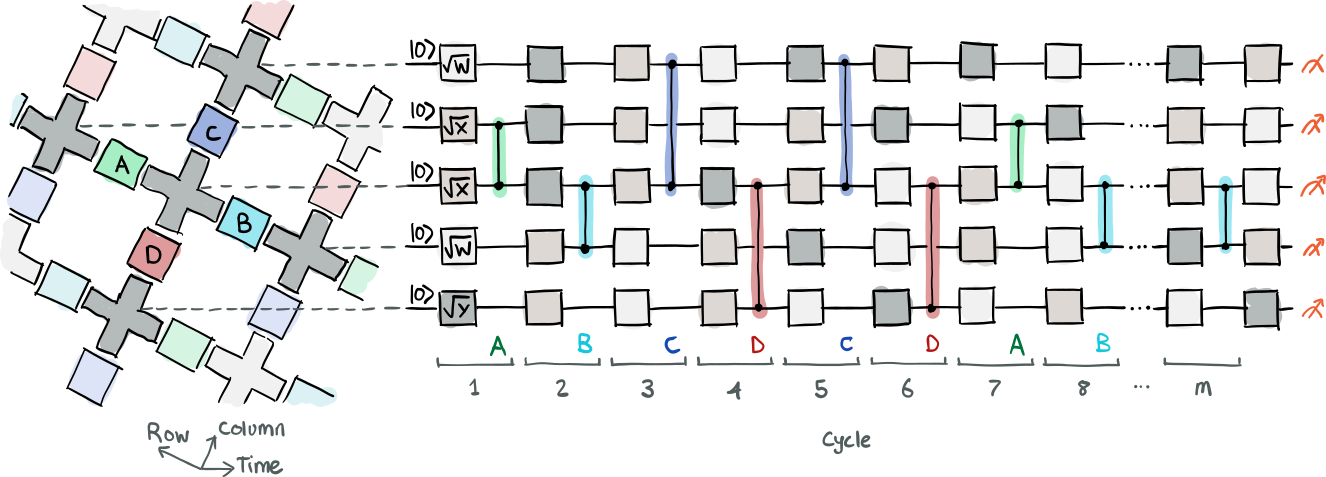
Here comes one of the tricky parts. To decide which qubits the two-qubit gates should be applied to, we have to look at how they are connected to each other. In an alternating pattern, each pair of neighbouring qubits gets labeled with a letter A-D, where A and B correspond to all horizontally neighbouring qubits (in a row), and C and D to the vertically neighbouring qubits (in a column). This is depicted in the figure below, where you can also see how the single-qubit gates are applied, as well as the cycles, each consisting of a layer of single-qubit gates and a pair of two-qubit gates. Note that each coloured two-qubit gate represented in the image is implemented as the two consecutive gates iSWAP and CPhase in this demo.

Image taken from Arute, F., Arya, K., Babbush, R. et al. 1

The logic below iterates through all connections and returns a dictionary, gate_order, where the keys are the connection labels between different qubits and the values are lists of all neighbouring qubit pairs. We will use this dictionary inside the circuit to iterate through the different pairs and apply the two two-qubit gates that we just defined above. The way we iterate through the dictionary will depend on a gate sequence defined in the next section.

from itertools import combinations

gate_order = {"A":[], "B":[], "C":[], "D":[]}
for i, j in combinations(qubits, 2):
    wire_1 = qb2wire[i]
    wire_2 = qb2wire[j]
    if i in j.neighbors():
        if i.row == j.row and i.col % 2 == 0:
            gate_order["A"].append((wire_1, wire_2))
        elif i.row == j.row and j.col % 2 == 0:
            gate_order["B"].append((wire_1, wire_2))
        elif i.col == j.col and i.row % 2 == 0:
            gate_order["C"].append((wire_1, wire_2))
        elif i.col == j.col and j.row % 2 == 0:
            gate_order["D"].append((wire_1, wire_2))

At this point we can define the gate sequence, which is the order the two-qubit gates are applied to the different qubit pairs. For example, ["A", "B"] would mean that the two-qubit gates are first applied to all qubits connected with label A, and then, during the next full cycle, the two-qubit gates are applied to all qubits connected with label B. This would then correspond to a 2-cycle run (or a circuit with a depth of 2).

While we can define any patterns we’d like, the two gate sequences below are the ones that are used in the paper. The shorter one is used for their classically verifiable benchmarking. The slightly longer sequence, which is much harder to simulate classically, is used for estimating the cross-entropy fidelity in what they call the “supremacy regime”. We will use the shorter gate sequence for the following demonstration; feel free to play around with other combinations.

m = 14  # number of cycles

gate_sequence_longer = np.resize(["A", "B", "C", "D", "C", "D", "A", "B"], m)
gate_sequence = np.resize(["A", "B", "C", "D"], m)

The single-qubit gates are randomly selected and applied to each qubit in the circuit, while avoiding the same gate being applied to the same wire twice in a row. We do this by creating a helper function generate_single_qubit_gate_list() that specifies the order in which the single-qubit gates should be applied. We can use this list within the circuit to know which gate to apply when.

def generate_single_qubit_gate_list():
    # create the first list by randomly selecting indices
    # from single_qubit_gates
    g = [list(np.random.choice(range(len(single_qubit_gates)), size=wires))]

    for cycle in range(len(gate_sequence)):
        g.append([])
        for w in range(wires):
            # check which gate was applied to the wire previously
            one_gate_removed = list(range(len(single_qubit_gates)))
            bool_list = np.array(one_gate_removed) == g[cycle][w]

            # and remove it from the choices of gates to be applied
            pop_idx = np.where(bool_list)[0][0]
            one_gate_removed.pop(pop_idx)
            g[cycle + 1].append(np.random.choice(one_gate_removed))
    return g

Finally, we can define the circuit itself and create a QNode that we will use for circuit evaluation with the qsim device. The two-qubit gates are applied to the qubits connected by A, B, C, or D as defined above. The circuit ends with a half-cycle, consisting of only a layer of single-qubit gates.

From the QNode, we need both the probabilities of the measurement results, as well as raw samples. To facilitate this, we add a keyword argument to our circuit allowing us to switch between the two returns. We take samples from the computational basis state using all wires, which will return bitstrings of values \(0\) and \(1\), corresponding to the states \(\left|0\right>\) and \(\left|1\right>\).

@qml.qnode(dev)
def circuit(seed=42, return_probs=False):
    np.random.seed(seed)
    gate_idx = generate_single_qubit_gate_list()

    # m full cycles - single-qubit gates & two-qubit gate
    for i, gs in enumerate(gate_sequence):
        for w in range(wires):
            single_qubit_gates[gate_idx[i][w]](wires=w)

        for qb_1, qb_2 in gate_order[gs]:
            qml.ISWAP(wires=(qb_1, qb_2))
            qml.CPhase(-np.pi/6, wires=(qb_1, qb_2))

    # one half-cycle - single-qubit gates only
    for w in range(wires):
        single_qubit_gates[gate_idx[-1][w]](wires=w)

    if return_probs:
        return qml.probs(wires=range(wires))
    else:
        return qml.sample()

The cross-entropy benchmarking fidelity

The performance metric that is used in the experiment, and the one that we will use in this demo, is called the linear cross-entropy benchmarking fidelity. It’s defined as

\[F_{XEB} = 2^{n}\left<P(x_i)\right> - 1,\]

where \(n\) is the number of qubits, \(P(x_i)\) is the probability of bitstring \(x_i\) computed for the ideal quantum circuit, and the average is over the observed bitstrings.

The idea behind using this fidelity is that it will be close to 1 for samples obtained from random quantum circuits, such as the one we defined above, and close to zero for a uniform probability distribution, which can be effectively sampled from classically. Sampling a bitstring from a random quantum circuit would follow the distribution

\[Pr(p) = (N - 1)(1- p)^{N-2},\]

where \(N = 2^n\) is the number of possible bitstrings 4. This distribution is approximated well by the Porter-Thomas distribution, given by \(Pr(p) = Ne^{-Np}\), a characteristic property of chaotic quantum systems. From this we can then calculate the expectation value \(\left<P(x_i)\right>\) as follows:

\[\left<P(x_i)\right> = \int_0^1 p^2 N (N-1)(1-p)^{N-2}dp = \frac{2}{N+1},\]

which leads to the theoretical fidelity

\[F_{XEB} = 2^{n}\left<P(x_i)\right> - 1 = \frac{2N}{N+1} - 1.\]

We implement this fidelity as the function below, where samples is a list of sampled bitstrings, and probs is a list with corresponding sampling probabilities for the same noiseless circuit.

def fidelity_xeb(samples, probs):
    sampled_probs = []
    for bitstring in samples:
        # convert each bitstring into an integer
        bitstring_idx = int(bitstring, 2)

        # retrieve the corresponding probability for the bitstring
        sampled_probs.append(probs[bitstring_idx])

    return 2 ** len(samples[0]) * np.mean(sampled_probs) - 1

We set a random seed and use it to calculate the probability for all the possible bitstrings. It is then possible to sample from exactly the same circuit by using the same seed. Before calculating the cross-entropy benchmarking fidelity, the Pauli-Z samples need to be converted into their correponding bitstrings, since we need the samples to be in the computational basis.

Note

Every time the previously defined circuit is run using the qsim device, qsimcirq will print a warning message because the circuit has no intermediate measurements. More information about this warning can be found in the Measurement sampling section of the qsimcirq guide.

seed = np.random.randint(0, 42424242)
probs = circuit(seed=seed, return_probs=True)
circuit_samples = circuit(seed=seed)

# get bitstrings from the samples
bitstring_samples = []
for sam in circuit_samples:
    bitstring_samples.append("".join(str(bs) for bs in sam))

f_circuit = fidelity_xeb(bitstring_samples, probs)

Similarly, we can sample random bitstrings from a uniform probability distribution by generating all basis states, along with their corresponding bitstrings, and sample directly from them using NumPy.

basis_states = dev.generate_basis_states(wires)
random_integers = np.random.randint(0, len(basis_states), size=shots)
bitstring_samples = []
for i in random_integers:
    bitstring_samples.append("".join(str(bs) for bs in basis_states[i]))

f_uniform = fidelity_xeb(bitstring_samples, probs)

Finally, let’s compare the two different values. Sampling from the circuit’s probability distribution should give a fidelity close to 1, while sampling from a uniform distribution should give a fidelity close to 0.

Note

The cross-entropy benchmarking fidelity may output values that are negative or that are larger than 1, for any finite number of samples. This is due to the random nature of the sampling. For an infinite amount of samples, or circuit runs, the observed values will tend towards the theoretical ones, and will then always lie in the 0-to-1 interval.

print("Circuit's distribution:", f"{f_circuit:.7f}".rjust(12))
print("Uniform distribution:", f"{f_uniform:.7f}".rjust(14))

Out:

Circuit's distribution:    1.0398803
Uniform distribution:      0.0013487

To show that the fidelity from the circuit sampling actually tends towards the theoretical value calculated above we can run several different random circuits, calculate their respective cross-entropy benchmarking fidelities and then calculate the mean fidelity of all the runs. The more evaluations we do, the closer to the theoretical value we should get.

In the experiment, they typically calculate each of their presented fidelities over ten circuit instances, which only differ in the choices of single-qubit gates. In this demo, we use even more instances to demonstrate a value closer to the theoretically obtained one.

Note

The following mean fidelity calculations can be interesting to play around with. You can change the qubit grid at the top of this demo using, e.g., 8 or 4 qubits; change the number of shots used; as well as the number of circuit evaluations below. Running the following code snippet, the mean fidelity should still tend towards the theoretical value (which will be lower for fewer qubits).

N = 2 ** wires
theoretical_value = 2 * N / (N + 1) - 1

print("Theoretical:", f"{theoretical_value:.7f}".rjust(24))

f_circuit = []
num_of_evaluations = 100
for i in range(num_of_evaluations):
    seed = np.random.randint(0, 42424242)

    probs = circuit(seed=seed, return_probs=True)
    samples = circuit(seed=seed)

    bitstring_samples = []
    for sam in samples:
        bitstring_samples.append("".join(str(bs) for bs in sam))

    f_circuit.append(fidelity_xeb(bitstring_samples, probs))
    print(f"\r{i + 1:4d} / {num_of_evaluations:4d}{' ':17}{np.mean(f_circuit):.7f}", end="")
print("\rObserved:", f"{np.mean(f_circuit):.7f}".rjust(27))

Out:

Theoretical:                0.9995118
Observed:                   0.9999512

Classical hardness

Why are we calculating this specific fidelity, and what does it actually mean if we get a cross-entropy benchmarking fidelity close to 1? This is an important question, containing one of the main arguments behind why this experiment is used to demonstrate “quantum supremacy”.

Much is due to the Porter-Thompson probability distribution that the random quantum circuits follow, which is hard to simulate classically. On the other hand, a quantum device, running a circuit as the one constructed above, should be able to sample from such a distribution without much overhead. Thus, by showing that a quantum device can produce a high enough fidelity value for a large enough circuit, “quantum supremacy” can be claimed. This is exactly what Google’s experiment has done.

There’s still one issue that hasn’t been touched on yet: the addition of noise in quantum hardware. Simply put, this noise will lower the cross-entropy benchmarking fidelity—the larger the circuit, the more noise there will be, and thus the lower the fidelity, with the fidelity approaching 0 as the noise increases. By calculating the specific single-qubit, two-qubit, and readout errors of the Sycamore chip, and using them to simulate a noisy circuit, the Google AI quantum team was able to compare the run-times with the output from their actual hardware device. This way, they managed to show that a significant speedup could be gained from using a quantum computer, and thus proclaimed “quantum supremacy” (see Fig. 4 in 1).

Note

For more reading on this, the original paper 1 is highly recommended (along with the suplementary information 2 if you want to dive deeper into the math and physics of the experiment). The blog post in 5, along with the accompanying GitHub repo, also provides a nice introduction to the cross-entropy benchmarking fidelity, and includes calculations highlighting the effects of added noise models.

References

1(1,2,3)

Arute, F., Arya, K., Babbush, R. et al. “Quantum supremacy using a programmable superconducting processor” Nature 574, 505-510 (2019).

2

Arute, F., Arya, K., Babbush, R. et al. Supplementary information for “Quantum supremacy using a programmable superconducting processor” arXiv:1910.11333 (2019)

3

Martinis, John M. et al. (2020), Quantum supremacy using a programmable superconducting processor, Dryad, Dataset

4

Boixo, S., Isakov, S.V., Smelyanskiy, V.N. et al. Characterizing quantum supremacy in near-term devices. Nature Phys 14, 595-600 (2018)

5

Sohaib, Alam M. and Zeng, W., Unpacking the Quantum Supremacy Benchmark with Python

About the author

Theodor Isacsson

Theodor is a quantum software engineer based in Vancouver. He's currently at D-Wave Systems, having previously worked on the quantum software stack at Xanadu, where he contributed to packages such as Strawberry Fields, The Walrus and PennyLane.

demos/qsim_beyond_classical

 

Download Python script

 

Download Notebook

 

View on GitHub