Trapped ion quantum computers

Author: Alvaro Ballon — Posted: 10 November 2021. Last updated: 26 August 2022.

The race for quantum advantage is on! A host of competitors are using different technologies to build a useful quantum computer. Some common approaches are **trapped ions, superconducting qubits, and photonics, among others. Discussing whether there is a superior framework leads to a neverending debate. All of them pose complex technological challenges, which we can only solve through innovation, inventiveness, hard work, and a bit of luck. It is difficult to predict whether these problems are solvable in a given timeframe. More often than not, our predictions have been wrong. Forecasting the winner of this race is not easy at all!

Here, we introduce trapped ion quantum computers. It is the preferred technology that research groups use at several universities around the world, and at research companies like Honeywell and IonQ. In particular, Honeywell has achieved a quantum volume of 128, the largest in the market! As the name suggests, the qubits are ions trapped by electric fields and manipulated with lasers. Trapped ions have relatively long coherence times, which means that the qubits are long-lived. Moreover, they can easily interact with their neighbours. Scalability is a challenge, but, as we will see, there are innovative ways to get around them.

After reading this demo, you will learn how trapped ion quantum computers prepare, evolve, and measure quantum states. In particular, you will gain knowledge on how single and multi-qubit gates are implemented and how we can simulate them using PennyLane. You will also identify the features that make trapped ion quantum computers an appropriate physical implementation, and where the technical challenges lie, in terms of DiVincenzo’s criteria (see box below). Finally, you will become familiar with the concepts required to understand recent articles on the topic and read future papers to keep up-to-date with the most recent developments.

Di Vincenzo’s criteria: In the year 2000, David DiVincenzo proposed a wishlist for the experimental characteristics of a quantum computer 1. DiVincenzo’s criteria have since become the main guideline for physicists and engineers building quantum computers:

1. Well-characterized and scalable qubits. Many of the quantum systems that we find in nature are not qubits, so we must find a way to make them behave as such. Moreover, we need to put many of these systems together.

2. Qubit initialization. We must be able to prepare the same state repeatedly within an acceptable margin of error.

3. Long coherence times. Qubits will lose their quantum properties after interacting with their environment for a while. We would like them to last long enough so that we can perform quantum operations.

4. Universal set of gates. We need to perform arbitrary operations on the qubits. To do this, we require both single-qubit gates and two-qubit gates.

5. Measurement of individual qubits. To read the result of a quantum algorithm, we must accurately measure the final state of a pre-chosen set of qubits.

How to trap an ion

Why do we use ions, i.e., charged atoms, as qubits? The main reason is that they can be contained (that is, trapped) in one precise location using electric fields. It is possible to contain neutral atoms using optical tweezers, but our focus is on ions, which can be contained using an electromagnetic trap. Ion traps are rather old technology: their history goes back to 1953 when Wolfgang Paul proposed his now-called Paul trap 2. For this invention, Paul and Dehmelt were awarded the 1989 Physics Nobel Prize, since it is used to make highly precise atomic clocks. Current trapped ion quantum computers extensively use the Paul trap, but Paul won the prize six years before such an application was proposed 3!

It is not easy to create electric fields that contain the ion in a tiny region of space. The ideal configuration of an electric field —also known as a potential— would look like this:

Confining potential

The potential should be interpreted as a wall that the ion must climb over to escape from a physical region. Positively charged ions will always roll down from regions of high potential to low potential. So if we can achieve an electric potential like the above, the ion should remain trapped in the pit. However, using the laws of electrostatics, we can show that it is impossible to create a confining potential with only static electric fields. Instead, they produce saddle-shaped potentials:

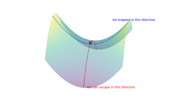
Saddle-shaped potential allowed by electrostatics

This potential is problematic since the ion is contained in one direction but could escape in the perpendicular direction. Therefore, the solution is to use time-dependent electric fields to allow the potential wall to move. What would happen, for example, if we rotated the potential plotted above? We can imagine that if the saddle potential rotates at a specific frequency, the wall will catch the ion as it tries to escape in the downhill direction. Explicitly, the electric potential that we generate is given by 4

\[\Phi = \frac{1}{2}\left(u_x x^2 + u_y y^2 + u_z z^2\right) + \frac{1}{2}\left(v_x x^2 + v_y y^2 + v_z z^2\right)\cos(\omega t+\phi).\]

The parameters \(u_i\), \(v_i\), and \(\phi\) need to be adjusted to the charge and mass of the ion and to the potential’s angular frequency \(\omega\). We have to tune these parameters very carefully, since the ion could escape if we do not apply the right forces at the right time. It takes a lot of care, but this technique is so old that it is almost perfect by now. Here is what the rotating potential would look like:

A rotating potential with the correct frequency and magnitude can contain an ion

We want to make a quantum computer, so having one qubit cannot be enough. We would like as many as we can possibly afford! The good news is that we have the technology to trap many ions and put them close together in a one-dimensional array, called an ion chain. Why do we need this particular configuration? To manipulate the qubits, we need the system of ions to absorb photons. However, shooting a photon at an ion can cause relative motion between ions. The proximity between qubits will cause unwanted interactions, which could modify their state. Happily, there is a solution to this issue: we place the ions in a sufficiently spaced one-dimensional array and cool them all down to the point where their motion in space is quantized. In this scenario, photons that would bring the ion to their excited states will not cause any relative motion. Instead, all ions will recoil together 5. This phenomenon is called the Mossbauer effect. We will see later that by carefully tuning the laser frequency, we can control both the excitations of the ions and the motion of the ion chain. This user-controlled motion is precisely what we need to perform quantum operations with two qubits.

Trapped ions as robust qubits

Now that we know how to trap ions, we would like to use them as qubits. Would any ion out there work well as a qubit? In fact, only a select few isotopes will do the trick. The reason is that our qubit basis states are the ground and excited states of an electron in the atom, and we need to be able to transition between them using laser light. Therefore, we would like the atom to have an excited state that is long-lived, and also one that we may manipulate using frequencies that lasers can produce. Thanks to semiconductor laser technology, we have a wide range of frequencies that we can use in the visible and infrared ranges, so getting the desired frequency is not too much of a problem. The best ions for our purposes are single-charged ions in Group II of the periodic table, such as Calcium-40, Beryllium-9, and Barium-138, commonly used in university laboratories 7. The rare earth Ytterbium-171 is used by IonQ and Honeywell. These elements have two valence electrons, but their ionized version only has one. The valence electron is not so tightly bound to the atom, so it is the one whose state we use to represent a qubit.

Atomic Physics Primer: Atoms consist of a positively charged nucleus and negative electrons around them. The electrons inhabit energy levels, which have a population limit. As the levels fill up, the electrons occupy higher and higher energy levels. But as long as there is space, electrons can change energy levels, with a preference for the lower ones. This can happen spontaneously or due to external influences.

When the lower energy levels are not occupied, the higher energy levels are unstable: electrons will prefer to minimize their energy and jump to a lower level on their own. What happens when an electron jumps from a high energy level to a lower one? Conservation of energy tells us that the energy must go somewhere. Indeed, a photon with an energy equal to the energy lost by the electron is emitted. This energy is proportional to the frequency (colour) of the photon.

Conversely, we can use laser light to induce the opposite process. When an electron is in a stable or ground state, we can use lasers with their frequency set roughly to the difference in energy levels, or energy gap, between the ground state and an excited state . If a photon hits an electron, it will go to that higher energy state. When the light stimulus is removed, the excited electrons will return to stable states. The time it takes them to do so depends on the particular excited state they are in since, sometimes, the laws of physics will make it harder for electrons to jump back on their own.

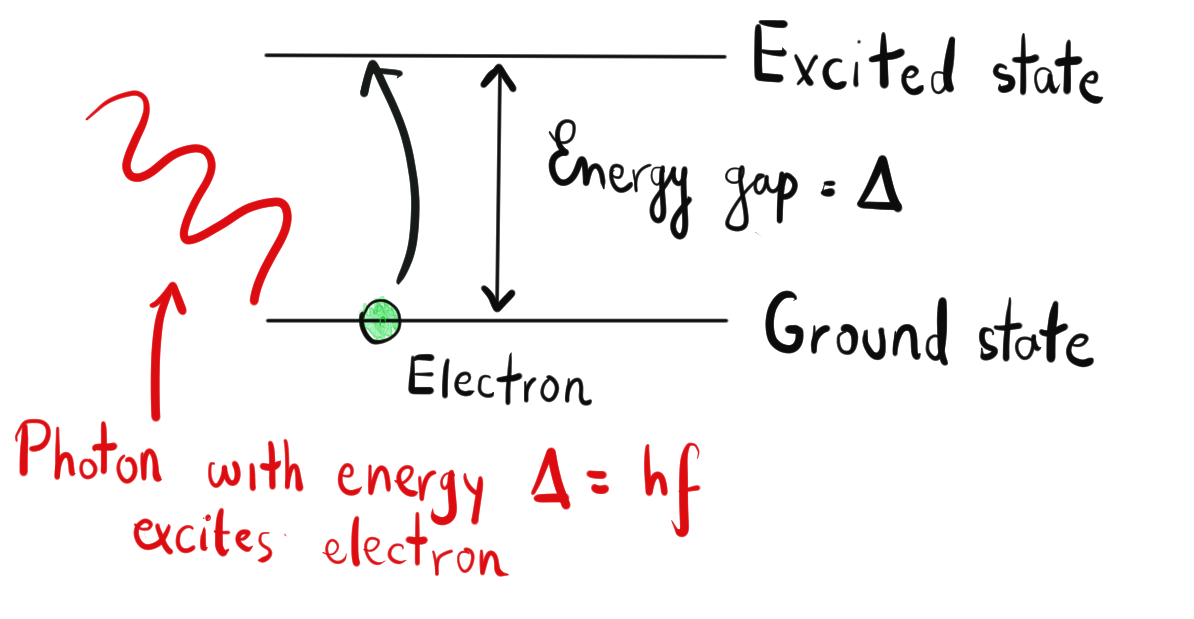
Photons with an energy equal to the atomic gap drive excitations

Having chosen the ions that will act as our qubits, we need to prepare them in a stable fiducial state, known as the ground state and denoted by \(\left\lvert g \right\rangle\). The preparation is done by a procedure called optical pumping. To understand how it works, let us take Calcium-40 as an example. In this case, the electron has two stable states with the same energy, but different direction of rotation. We denote these by \(\left\lvert g_1 \right\rangle\) and \(\left\lvert g_2\right\rangle\). We do not know which stable state the electron is in, and we would like to ensure that the electron is in the \(\left\lvert g_1\right\rangle\) state. This will be our chosen fiducial state, so \(\left\lvert g\right\rangle = \left\lvert g_1\right\rangle\). However, quantum mechanics forbids a direct transition between these two stable states. To get from one state to the other, the electron would have to change its rotation without giving out any energy, which is impossible! But we can take a detour: we use circularly polarized laser light of a particular wavelength (397nm for Calcium-40) to excite \(\left\lvert g_2\right\rangle\) into a short-lived excited state \(\left\lvert \textrm{aux}\right\rangle\). This light does not stimulate any other transitions in the ion so that an electron in the ground state \(\left\lvert g_1\right\rangle\) will remain there. Quantum mechanics tells us that, in a matter of nanoseconds, the excited electron decays to our desired ground state \(\left\lvert g \right\rangle\) with probability 1/3, but returns to \(\left\lvert g_2 \right\rangle\) otherwise. For this reason, we need to repeat the procedure many times, gradually “pumping” the electrons in all (or the vast majority of) our ions to the ground state.

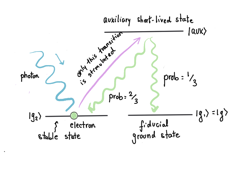
Optical pumping to prepare the ground state

What about the other basis qubit state? It will be a long-lived excited state, denoted by \(\left\lvert e \right\rangle\). For the Calcium-40 ion, this state is a metastable state: a state that has a sufficiently long lifetime since quantum mechanics restricts, but does not entirely forbid, transitions to a lower energy level. For example, the metastable state of Calcium-40 has a half-life of about 1 second. While apparently short, most quantum operations can be performed on a timescale of micro to milliseconds. The energy difference between the ground and excited state corresponds to a laser frequency of 729nm, achievable with an infrared laser. Therefore, we call this an optical qubit. An alternative is to use an ion, such as Calcium-43, that has a hyperfine structure, which means that the ground and excited states are separated by a very small energy gap. In this case, the higher energy state has a virtually infinite lifespan, since it is only slightly different from the stable ground state. We can use a procedure similar to optical pumping to transition between these two states, so while coherence times are longer for these hyperfine qubits, gate implementation is more complicated and needs a lot of precision.

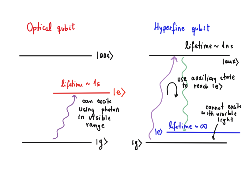
Optical vs. hyperfine qubits

We have now learned how trapped ions make for very stable qubits that allow us to implement many quantum operations without decohering too soon. We have also learned how to prepare these qubits in a stable ground state. Does this mean that we have already satisfied DiVincezo’s first, second, and third criteria? We have definitely fulfilled the second one since optical pumping is a very robust method. However, we have mainly been focusing on a single qubit and, since we have not discussed scalability yet, we have not fully satisfied the first criterion. Introducing more ions will pose additional challenges to meeting the third criterion. For now, let us focus on how to satisfy criteria 4 and 5, and we will come back to these issues once we discuss what happens when we deal with multiple ions.

Non-demolition measurements

Let us now discuss the last step in a quantum computation: measuring the qubits. Since it takes quite a bit of work to trap an ion, it would be ideal if we could measure the state of our qubits without it escaping from the trap. We definitely do not want to trap ions again after performing one measurement. Moreover, we want measurements that can be repeated on the same ions and yield consistent results. These are called non-demolition measurements, and they are easy enough to carry out for trapped ions.

The measurement method uses a similar principle to that of optical pumping. Once again, and continuing with the Calcium-40 example, we make use of the auxiliary state. This time, we shine a laser light wavelength of 397 nm that drives the transition from \(\left\lvert g \right\rangle\) to the auxiliary state \(\left\lvert \textrm{aux} \right\rangle\). The transition is short-lived; it will quickly go back to \(\left\lvert g \right\rangle\), emitting a photon of the same wavelength. The state \(\left\lvert e \right\rangle\) is not affected. Therefore, we will measure \(\left\lvert g \right\rangle\) if we see the ion glowing: it continuously emits light at a wavelength of 397 nm. Conversely, if the ion is dark, we will have measured the result corresponding to state \(\left\lvert e\right\rangle\). To see the photons emitted by the ions, we need to collect the photons using a lens and a photomultiplier, a device that transforms weak light signals into electric currents.

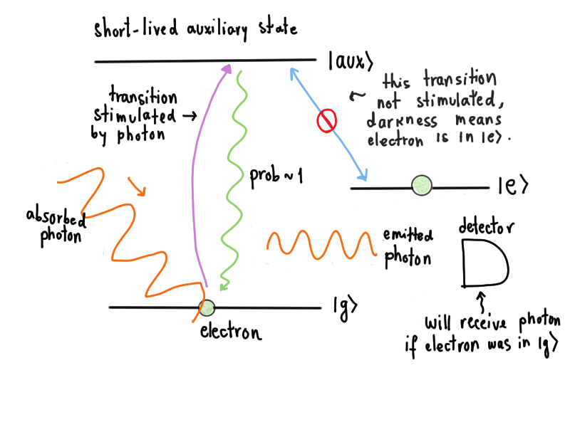
Non-demolition measurement of ion states

Have we fully satisfied the fifth criterion? Via a careful experimental arrangement, we can detect the emission of photons of each atom individually, so we are on the right track. But in reality, there is also some uncertainty in the measurement. In many quantum computing algorithms, we only measure the state of a pre-chosen set of ions called the ancilla. If these ions emit light, they can accidentally excite other ions on the chain, causing decoherence. A way to avoid this source of uncertainty is to use two species of ions: one for the ancilla and one for the qubits that are not measured, or logical qubits. In this case, the ions emitted by the ancilla ions would not excite the logical qubits. However, using two different species of ions causes extra trouble when we want to implement arbitrary qubit operations 6.

Rabi oscillations to manipulate single qubits

How do we make single-qubit quantum gates? Namely, is there a way to put the electron in a superposition of the ground and excited states? Since we aim to change the energy state of an electron, we have no choice but to continue using lasers to shoot photons at it, tuning the frequency to the energy gap. To understand how we would achieve a superposition by interacting with the ion using light, let us look at a mathematical operator called the Hamiltonian. In physics, the Hamiltonian describes the motion and external forces around an object we want to study. One of the main difficulties encountered in quantum mechanics is determining the correct Hamiltonian for a system. In our case, this work has already been done by quantum optics experts. After many simplifications involving some approximations, we find that the Hamiltonian that describes an electron in an ion resonant to the laser light is given by the operator

\[\hat{H}=\frac{\hbar\Omega}{2}\left(S_+ e^{i\varphi}+S_{-}e^{-i\varphi}\right).\]

Here, \(\Omega\) is the Rabi frequency. It is defined by \(\Omega=\mu_m B/2\hbar\), where \(B\) is the applied magnetic field due to the laser, and \(\mu_m\) is the magnetic moment of the ion. The phase \(\varphi\) measures the initial displacement of the light wave at the atom’s position. The matrices \(S_+\) and \(S_-\) are

\[\begin{split}S_+=\left( \begin{array}{cc} 0 & 0 \\ 1 & 0\end{array}\right), \qquad S_-=\left( \begin{array}{cc} 0 & 1 \\ 0 & 0\end{array}\right).\end{split}\]

Hamiltonians in physics are helpful because they tell us how systems change with time in the presence of external interactions. In quantum mechanics, Hamiltonians are represented by matrices, and the evolution of a system is calculated using Schrödinger’s equation. When the Hamiltonian does not depend on time, a qubit starting in state \(\left\lvert g \right\rangle\) will evolve into the following time-dependent state:

\[\left\lvert \psi(t)\right\rangle = \exp(-i \hat{H} t/\hbar)\left\lvert g \right\rangle,\]

where \(\exp\) denotes the matrix exponential and \(t\) is the duration of the interaction, which is controlled using pulses, i.e., short bursts of light. We do not need to elaborate on how matrix exponentials are calculated, since we can implement them using the scipy library in Python. Let us see how our basis states \(\left\lvert g \right\rangle\) and \(\left\lvert e \right\rangle\) (\(\left\lvert 0 \right\rangle\) and \(\left\lvert 1 \right\rangle\) in PennyLane) evolve under the action of this Hamiltonian. First, we write a function that returns the matrix exponential \(\exp(-i \hat{H} t/\hbar)\) as a function of \(\varphi\) and the duration \(t\) of the pulse, with \(\Omega\) set to 100 kHz.

import pennylane as qml
from pennylane import numpy as np
from scipy.linalg import expm

Omega = 100
S_plus = np.array([[0, 0], [1, 0]])
S_minus = np.array([[0, 1], [0, 0]])


def evolution(phi, t):
    Ham = Omega / 2 * (S_plus * np.exp(1j * phi) + S_minus * np.exp(-1j * phi))
    return expm(-1j * Ham * t)

With this operator implemented, we can determine the sequences of pulses that produce common gates. For example, there is a combination of pulses with different phases and durations that yield the Hadamard gate:

dev = qml.device("default.qubit", wires=1)


@qml.qnode(dev, interface="autograd")
def ion_hadamard(state):

    if state == 1:
        qml.PauliX(wires=0)

    """We use a series of seemingly arbitrary pulses that will give the Hadamard gate.
    Why this is the case will become clear later"""

    qml.QubitUnitary(evolution(0, -np.pi / 2 / Omega), wires=0)
    qml.QubitUnitary(evolution(np.pi / 2, np.pi / 2 / Omega), wires=0)
    qml.QubitUnitary(evolution(0, np.pi / 2 / Omega), wires=0)
    qml.QubitUnitary(evolution(np.pi / 2, np.pi / 2 / Omega), wires=0)
    qml.QubitUnitary(evolution(0, np.pi / 2 / Omega), wires=0)

    return qml.state()

#For comparison, we use the Hadamard built into PennyLane
@qml.qnode(dev, interface="autograd")
def hadamard(state):

    if state == 1:
        qml.PauliX(wires=0)

    qml.Hadamard(wires=0)

    return qml.state()

#We confirm that the values given by both functions are the same up to numerical error
print(np.isclose(1j * ion_hadamard(0), hadamard(0)))
print(np.isclose(1j * ion_hadamard(1), hadamard(1)))

Out:

[ True  True]
[ True  True]

Note that the desired gate was obtained up to a global phase factor. A similar exercise can be done for the \(T\) gate:

@qml.qnode(dev, interface="autograd")
def ion_Tgate(state):

    if state == 1:
        qml.PauliX(wires=0)

    qml.QubitUnitary(evolution(0, -np.pi / 2 / Omega), wires=0)
    qml.QubitUnitary(evolution(np.pi / 2, np.pi / 4 / Omega), wires=0)
    qml.QubitUnitary(evolution(0, np.pi / 2 / Omega), wires=0)

    return qml.state()


@qml.qnode(dev, interface="autograd")
def tgate(state):

    if state == 1:
        qml.PauliX(wires=0)

    qml.T(wires=0)

    return qml.state()


print(np.isclose(np.exp(1j * np.pi / 8) * ion_Tgate(0), tgate(0)))
print(np.isclose(np.exp(1j * np.pi / 8) * ion_Tgate(1), tgate(1)))

Out:

[ True  True]
[ True  True]

This PennyLane code shows that we can obtain a Hadamard gate and a \(T\) gate using consecutive pulses with different times and phases. Namely, to get a Hadamard gate, we need five pulses, all of them with duration \(t=\frac{\pi}{2\Omega}\), where the second and the fourth pulse have a phase of \(\pi/2\). The Hadamard and \(T\) gates together can be used to implement any operation on a single qubit, to an arbitrary degree of approximation. We see that timing and dephasing our laser pulses provides a versatile way to manipulate single qubits.

To get a better idea about how the duration of the pulses affects the state that we generate, let us plot the probability of obtaining the state \(\left\lvert e \right\rangle\) against the duration of the pulse for a fixed phase of \(\varphi = 0\).

import matplotlib.pyplot as plt


@qml.qnode(dev, interface="autograd")
def evolution_prob(t):

    qml.QubitUnitary(evolution(0, t / Omega), wires=0)

    return qml.probs(wires=0)


t = np.linspace(0, 4 * np.pi, 101)
s = [evolution_prob(i)[1].numpy() for i in t]

fig1, ax1 = plt.subplots(figsize=(9, 6))

ax1.plot(t, s, color="#9D2EC5")

ax1.set(
    xlabel="time (in units of 1/Ω)",
    ylabel="Probability",
    title="Probability of measuring the excited state"
)
ax1.grid()

plt.show()

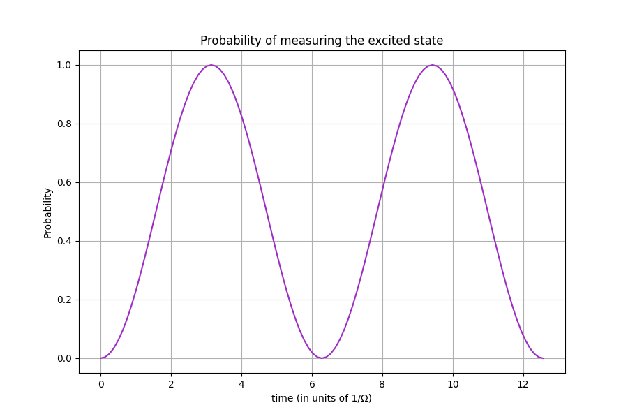
We see that the probability of obtaining the excited state changes with the duration of the pulse, reaching a maximum at a time \(t=\pi/\Omega\), and then vanishing at \(t=2\pi/\Omega\). This pattern keeps repeating itself and is known as a Rabi oscillation.

In fact, we can solve the Schrödinger equation explicitly (feel free to do this if you want to practice solving differential equations!). If we do this, we can deduce that the ground state \(\left\lvert g \right\rangle\) evolves to 7

\[\left\lvert \psi_0(t) \right\rangle = \cos\left(\frac{\Omega t}{2}\right)\left\lvert g \right\rangle -i\sin\left(\frac{\Omega t}{2}\right) e^{i\varphi}\left\lvert e \right\rangle .\]

We observe that we can obtain an arbitrary superposition of qubits by adjusting the duration of the interaction and the phase. This means that we can produce any single-qubit gate! To be more precise, let us see what would happen if the initial state was \(\left\lvert e \right\rangle\). As before, we can show that the evolution is given by

\[\left\lvert \psi_1(t) \right\rangle = -i\sin\left(\frac{\Omega t}{2}\right)e^{-i\varphi}\left\lvert g \right\rangle +\cos\left(\frac{\Omega t}{2}\right)\left\lvert e \right\rangle .\]

Therefore, the unitary induced by a laser pulse of amplitude \(B\), duration \(t\), and phase \(\varphi\) on an ion with magnetic moment \(\mu_m\) is

\[\begin{split}U(\Omega,\varphi,t)=\left( \begin{array}{cc} \cos\left(\frac{\Omega t}{2}\right) & -i\sin\left(\frac{\Omega t}{2}\right)e^{-i\varphi} \\ -i\sin\left(\frac{\Omega t}{2}\right)e^{i\varphi} & \cos\left(\frac{\Omega t}{2}\right)\end{array}\right),\end{split}\]

which has the form of a general rotation. Since we can generate arbitrary X and Y rotations using \(\varphi=0\) and \(\varphi=\pi/2\), Rabi oscillations allow us to build a universal set of single-qubit gates.

Achieving the required superpositions of quantum states requires precise control of the timing and phase of the pulse. This feat is not easy, but it is not the most challenging step towards creating a trapped-ion quantum computer. For typical Rabi frequencies of \(\Omega=100\) kHz, the single-qubit gates can be implemented in a few milliseconds with high accuracy. Thus, we can implement quantum algorithms involving many gates even for the seemingly short lifespans of optical qubits. As a consequence, we have now satisfied the single-qubit gate requirement of criterion 4. The rest of this criterion is not theoretically difficult to implement. However, it can be experimentally challenging.

The ion chain as a harmonic oscillator

To fully address the fourth criterion, we need to create gates on two qubits. How can we achieve this? It turns out that placing ions in a chain is ideal for multiple-qubit gate implementations. When cooled down, the entire ion chain acts as a quantum harmonic oscillator, meaning that it can vibrate with energies that are multiples of Planck’s constant \(\hbar\) times a fundamental frequency \(\omega\):

\[E=n\hbar\omega.\]

When the chain is oscillating with energy \(E=n\hbar\omega\), we denote the harmonic oscillator state, also known as phonon state or motional state, by \(\left\lvert n\right\rangle\). The harmonic oscillator can absorb and emit energy in multiples of \(\hbar\omega\), in packets of energy known as phonons. When we shine laser light on a particular atom of the ion chain, the entire chain could absorb the energy of the photons and start oscillating. However, we have seen that this does not happen when the atoms are cooled down and the light frequency matches the energy gap. Instead, the atom changes energy level, and we can manipulate a single qubit. But what happens when the frequency is away from this value? In most cases, it does nothing, but it will excite both the atom and the harmonic oscillator in some special circumstances. We can use the harmonic oscillator states as auxiliary states that will allow us to build two-qubit gates.

Let us introduce some notation that will help us understand exactly how the two-qubit gates are implemented. When an ion is in the ground state \(\left\lvert g \right\rangle\) and the chain is in the state \(\left\lvert n \right\rangle\), we will write the state as \(\left\lvert g \right\rangle \left\lvert n \right\rangle\), and similarly when the ion is in the excited state \(\left\lvert e \right\rangle\). If we are studying two ions at the same time, then we will write the states in the form \(\left\lvert g \right\rangle\left\lvert g \right\rangle\left\lvert n \right\rangle\), where the last \(\left\lvert n \right\rangle\) always represents the state of the oscillating ion chain. Suppose that the ion’s energy gap value is \(\Delta\), and we shine light of frequency \(\omega_b=\omega+\Delta\) on a particular ion. If it is in the ground state, it will absorb an energy \(\Delta\), and the ion chain will absorb the rest. Therefore, this light frequency induces the following blue sideband transition:

\[\left\lvert g \right\rangle \left\lvert n \right\rangle \rightarrow \left\lvert e \right\rangle \left\lvert n+1\right\rangle.\]

By using the frequency \(\omega_r=\Delta-\omega\), we can instead excite the ion and de-excite the ion chain, also known as a red sideband transition:

\[\left\lvert g \right\rangle \left\lvert n \right\rangle \rightarrow \left\lvert e \right\rangle \left\lvert n-1\right\rangle.\]

Crucially, this frequency will do nothing if the ion chain is in the state of zero energy. If the light frequency is exactly \(\Delta\), the ion chain does not absorb any phonons, but the ion does become excited. We will call this a carrier transition.

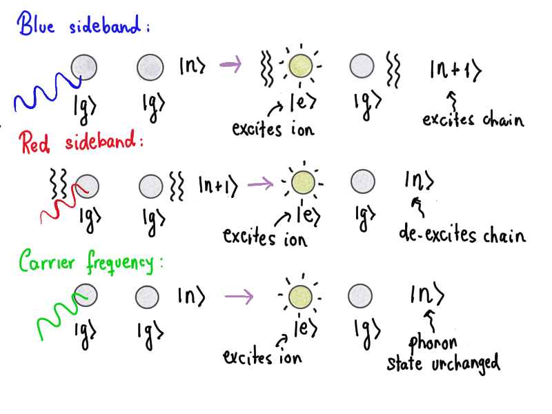
Effects of the sideband and carrier frequencies on an ion chain

Since the oscillations of the ion chain are quantum states, we may wonder whether we can also create superpositions of motional states. For both the red and blue sideband frequencies, the Hamiltonian turns out to be similar to the one we saw above, but with a different Rabi frequency \(\tilde{\Omega}\). Following the same prescription as with single ions, we can tune the duration and phase of the pulses to form superpositions of phonon states. For example, for a blue sideband pulse of duration \(t=\pi/2\tilde{\Omega}\) and phase \(\varphi=\pi/2\), a system of two ions in both the motional and electronic ground state evolves as

\[\left\lvert g\right\rangle \left\lvert g\right\rangle \left\lvert n\right\rangle \rightarrow \frac{1}{\sqrt{2}}\left(\left\lvert g\right\rangle \left\lvert g\right\rangle \left\lvert n\right\rangle + \left\lvert e\right\rangle \left\lvert g\right\rangle \left\lvert n+1\right\rangle\right)\]

when the pulse is incident on the first ion. Similarly, other choices of duration and phase allow for arbitrary superpositions between phonon states. This freedom to act on the motional states gives us the necessary tools to implement two-qubit gates. We will see two examples and use one of them to build a CNOT gate which, as is well-known, allows for universal computations when combined with single-qubit gates.

Note

The results above are relatively simple to understand, but they are not exact. In particular, to guarantee that the sideband frequencies will have the effects we described on the ion chain, the separation between ions must be large enough, in a range known as the Lamb-Dicke regime. If we do not operate under this condition, stronger interactions will come into play, and we will not be able to act on individual ions with the laser beams.

Entangling ions with multi-qubit gates

Maximally entangled states: When all outcomes have the same probability in an entangled state, such as in the two-ion state

\[\left\lvert \psi \right\rangle = \frac{1}{\sqrt{2}}\left(\left\lvert e \right\rangle \left\lvert g \right\rangle + \left\lvert g \right\rangle \left\lvert e \right\rangle\right),\]

we say that it is maximally entangled. To be able to do arbitrary computations and for quantum advantage to be possible, we need two-qubit gates that, combined with single qubit gates, produce maximally entangled states. The CNOT gate is an example of this, and we will learn about others below.

The Cirac-Zoller gate 3 can completely entangle ions. It is also the simplest way to illustrate how we can use the states of the harmonic oscillator as an aid to create two-qubit gates. For a chain with zero motional energy, we saw above that applying a blue sideband pulse of duration \(t=\pi/2\tilde{\Omega}\) and phase \(\varphi=\pi/2\) to the first ion gives us the state

\[\left\lvert \psi \right\rangle = \frac{1}{\sqrt{2}}\left(\left\lvert g\right\rangle \left\lvert g\right\rangle \left\lvert 0\right\rangle + \left\lvert e\right\rangle \left\lvert g\right\rangle \left\lvert 1\right\rangle\right).\]

We can then use a similar idea to keep creating superpositions until we end up in a maximally entangled state. The steps to implement the Cirac-Zoller gate are shown on the diagram:

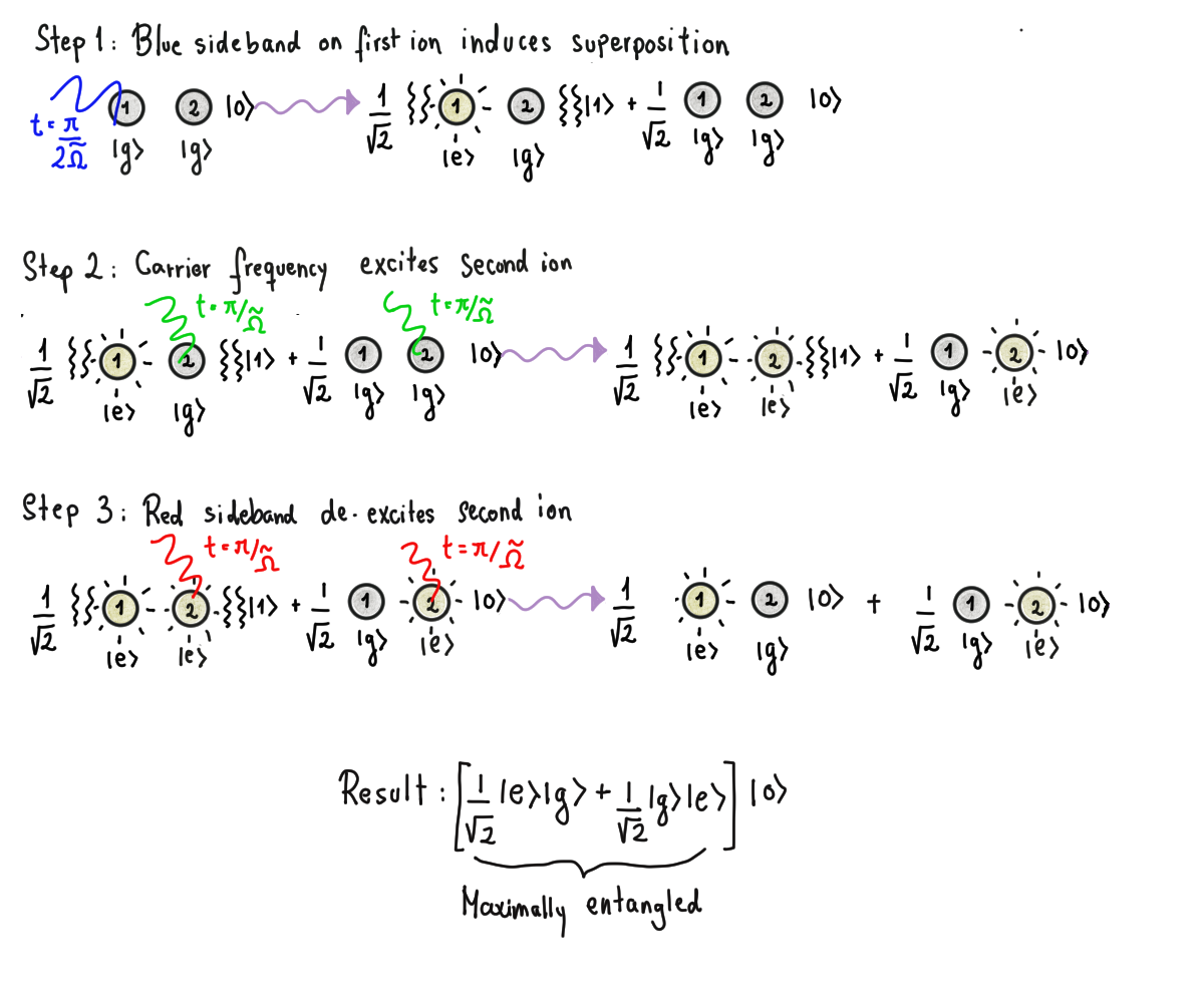
Implementation of the Cirac-Zoller gate using phonon states

We see that the consecutive application of a blue sideband, a carrier frequency, and a red sideband, with different durations, gives us a maximally entangled state. It is important to note that, in the last step, the part of the superposition that has no chain motion is unaffected by the red sideband. This property allows the creation of entanglement in electronic states by using the phonon states.

However, the implementation of the Cirac-Zoller gate in real life is plagued by problems. First, the ion chain needs to be completely cooled down to the ground motional state, which can never be achieved. Second, the gate is too slow. Surely, if we use hyperfine qubits, we can take as long as we want to implement the gates. The problem comes from the harmonic oscillator states. Since ion chains are large and less isolated from the environment, phonon states are rather short-lived due to decoherence.

For actual applications, we use a more ingenious gate, known as the Mølmer-Sørensen gate 8. It has the advantage that the ions do not need to be perfectly cooled to the motional ground state for it to work. It relies on simultaneously shining two lasers at different frequencies \(\omega_{\pm}\) on the two target ions, which are slightly detuned from the atomic energy gap \(\Delta\):

\[\omega_{\pm}=\Delta \pm \delta\]

The net effect of this interaction with laser light is to excite \(\left\lvert g \right\rangle \left\lvert g \right\rangle \left\lvert n \right\rangle \rightarrow \left\lvert e \right\rangle \left\lvert e \right\rangle\left\lvert n \right\rangle\), and it can do so through any of the four paths shown below:

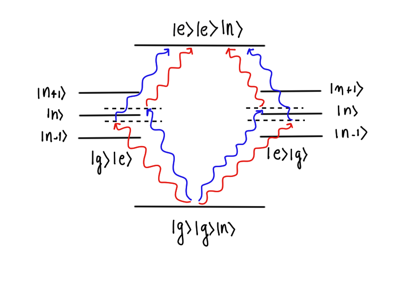
Mølmer-Sørensen gate implemented with two simultaneous laser pulses

Using a quantum mechanical technique known as perturbation theory, we can deduce that there is also a Rabi frequency \(\Omega_{MS}\) associated with this evolution. Therefore, adjusting the time and the phase of the lasers can lead to a superposition of \(\left\lvert g \right\rangle \left\lvert g \right\rangle \left\lvert n \right\rangle\) and \(\left\lvert e \right\rangle \left\lvert e \right\rangle\left\lvert n \right\rangle\). For example, we can obtain the state \(\frac{1}{\sqrt{2}}\left(\left\lvert g \right\rangle \left\lvert g \right\rangle\left\lvert n \right\rangle +\left\lvert e \right\rangle \left\lvert e \right\rangle\left\lvert n \right\rangle\right)\) which, in the two-ion subsystem, corresponds to the maximally entangled state \(\frac{1}{\sqrt{2}}\left(\left\lvert g \right\rangle \left\lvert g \right\rangle +\left\lvert e \right\rangle \left\lvert e \right\rangle\right)\). Using Schrödinger’s equation allows us to derive how the qubits evolve when we apply the Mølmer-Sørensen protocol for a time \(t\). The Hamiltonian is more involved, so we will not do this. We simply state the result (for zero phase) and implement it via a Python function

\[\begin{split}U_{MS}(t) =\left( \begin{array}{cccc} \cos(\frac{\Omega_{MS}t}{2}) & 0 & 0 & -i\sin(\frac{\Omega_{MS} t}{2})\\ 0 & \cos(\frac{\Omega_{MS} t}{2}) & -i\sin(\frac{\Omega_{MS} t}{2}) & 0 \\ 0 & -i\sin(\frac{\Omega_{MS} t}{2}) & \cos(\frac{\Omega_{MS} t}{2}) & 0 \\ -i\sin(\frac{\Omega_{MS} t}{2}) & 0 & 0 & \cos(\frac{\Omega_{MS} t}{2}) \end{array} \right)\end{split}\]

Omega = 100


def Molmer_Sorensen(t):
    ms = np.array(
        [
            [np.cos(Omega * t / 2), 0, 0, -1j * np.sin(Omega * t / 2)],
            [0, np.cos(Omega * t / 2), -1j * np.sin(Omega * t / 2), 0],
            [0, -1j * np.sin(Omega * t / 2), np.cos(Omega * t / 2), 0],
            [-1j * np.sin(Omega * t / 2), 0, 0, np.cos(Omega * t / 2)],
        ]
    )
    return ms

Since the CNOT gate is commonly used in quantum algorithms, let us determine how to obtain it from the Mølmer-Sørensen gate. It is possible to do so by using a combination of single-qubit rotations and the Mølmer-Sørensen gate applied for a period of \(t=\pi/2\Omega_{MS}\). Explicitly, we do this using the following circuit 9:

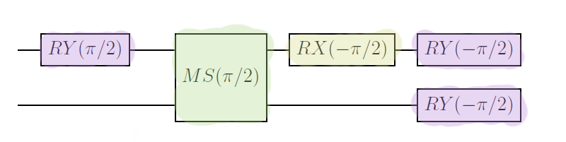
Circuit for the CNOT gate using rotations and an MS gate

where \(RX\) and \(RY\) are the usual rotations around the X and Y axes, and \(MS(t)\) denotes the Mølmer-Sørensen gate applied for a time \(t/\Omega_{MS}\). Let us verify that this is indeed the case by building the circuit in PennyLane:

dev2 = qml.device("default.qubit",wires=2)

@qml.qnode(dev2, interface="autograd")
def ion_cnot(basis_state):

    #Prepare the two-qubit basis states from the input
    qml.templates.BasisStatePreparation(basis_state, wires=range(2))

    #Implements the circuit shown above
    qml.RY(np.pi/2, wires=0)
    qml.QubitUnitary(Molmer_Sorensen(np.pi/2/Omega),wires=[0,1])
    qml.RX(-np.pi/2, wires=0)
    qml.RX(-np.pi/2, wires=1)
    qml.RY(-np.pi/2, wires=0)

    return qml.state()

#Compare with built-in CNOT
@qml.qnode(dev2, interface="autograd")
def cnot_gate(basis_state):

    qml.templates.BasisStatePreparation(basis_state, wires=range(2))

    qml.CNOT(wires=[0,1])

    return qml.state()

#Check that they are the same up to numerical error and global phase
print(np.isclose(np.exp(-1j*np.pi/4)*ion_cnot([0,0]),cnot_gate([0,0])))
print(np.isclose(np.exp(-1j*np.pi/4)*ion_cnot([0,1]),cnot_gate([0,1])))
print(np.isclose(np.exp(-1j*np.pi/4)*ion_cnot([1,0]),cnot_gate([1,0])))
print(np.isclose(np.exp(-1j*np.pi/4)*ion_cnot([1,1]),cnot_gate([1,1])))

Out:

[ True  True  True  True]
[ True  True  True  True]
[ True  True  True  True]
[ True  True  True  True]

This is indeed the CNOT gate, up to a global phase. At sufficiently low temperatures, the Rabi frequency \(\Omega_{MS}\) does not depend on the initial harmonic oscillator state, so this method can be used reliably even when we fail to cool down the ion chain completely. This property also makes this gate more robust to the decoherence of the chain.

The problem with too many ions

We have learned that the trapped ion paradigm allows us to prepare and measure individual qubits, and that we can implement single and multi-qubit gates with high accuracy. What’s not to like? As in every physical realization of quantum computers, trapped ions come with advantages and disadvantages. The main problem shared by all physical implementations of quantum computers is scalability. The root of the problem and the technological challenges involved depend on our particular framework.

To understand why scalability is a problem for trapped ions, let us consider a long ion chain. As discussed in the previous section, to implement multi-qubit gates, we need to lean on the harmonic oscillator states of the ion chains. These turn out to be a blessing and a curse simultaneously. Quantum computing with trapped ions would not be possible without motional states. However, if we put more ions in the chain, the values of the frequencies needed to excite it become too close together. As a consequence, unless we are extremely careful with our laser frequencies, we may end up in the wrong quantum state. We do not have infinite precision, so when the number of ions becomes close to 100, our current gate technology becomes practically unusable.

Is there a way to make the frequency values more spread out? One way is to reduce the Rabi frequency of the Mølmer-Sørensen gate, which we control by changing the strength of the laser light. Disappointingly, not only does this strategy make it harder to control the ion, but it also increases the time needed to apply the Mølmer-Sørensen gate. As already mentioned in the previous section, time is of the essence when applying multi-qubit gates since the motional states of the chain are extremely sensitive to decoherence. We cannot afford to have even slower gates.

Which of the DiVincenzo criteria do trapped ions quantum computers still fail to meet? Criterion 1 is only met partially: we do have robust qubits, but there seems to be a hard technological limit for scalability. Criterion 3 also becomes an issue when the ion chain is too long since coherence times for motional states become shorter. The two-qubit requirement of criterion 4 is related to this decoherence problem since multi-qubit gates can take too long to implement accurately in a long ion chain. Criterion 2, as already discussed, does not present too much of a problem thanks to optical pumping technology. However, problems remain for criterion 5. As we already saw, we can use two different species of ions to obtain good measurements. But, in general, it is challenging to implement consecutive good-quality two-qubit gates between different ion species; strategies like the Mølmer-Sørensen gate will not work and need modification.

The state of the art

Of course, no matter how insurmountable these challenges seem to be, physicists will not give up. Many ingenious ways to address these technical complications have already been proposed. Not surprisingly, it is one of the hottest research topics in quantum computing, and papers with newer technologies have probably been published since this tutorial was written.

The main issue discussed above is that a long ion chain is noisy and makes qubits challenging to manipulate. In 2002, Kielpinski and collaborators 11 came up with an intelligent solution: if size is a problem, let us make the chain shorter! Of course, we would still like to be able to manipulate thousands of qubits. To achieve this, we could build a segmented trap, also known as a QCCD (Quantum Charge-Coupled Device) architecture. The idea is to make our traps mobile. We could move ions from one place to another whenever we need to apply a multi-qubit gate and move them far away when we need to manipulate them individually. Thus, the chain that we interact with when we need to entangle qubits is not long. This method makes the motional states less prone to decoherence. The phonon frequencies are also sufficiently spread apart so that the gates can be implemented.

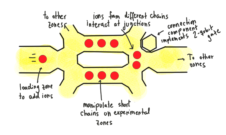
Example of a proposed QCCD architecture, as in 12

QCCD architectures sound like a straightforward solution, but seeing as we do not have large quantum computers yet, there must be some nuances. In practice, moving ions around a trap is not easy at all. The containing potential must be changed in a highly accurate manner to transport the ions without losing them. Such technology has not been perfected yet. While it has been possible to manipulate ions and make them interact, the traps we need for a good quantum computer are somewhat involved. We want multiple segments in the trap that allow for arbitrary ions to be brought together to run quantum algorithms without any limitations. In April 2021, Honeywell reported building a multi-segment QCCD architecture with six qubits and two interaction zones 13. However, it is unclear how this proposed technology would scale to higher orders of magnitude.

Another path towards a solution would be to simply accept the short coherence times of the ion chains, and try to make the two-qubit gates faster. Such an approach is being followed by the startup IonQ. In January 2021, they showed that it is possible to speed up the Mølmer-Sørensen gate by one order of magnitude by changing the shape of the laser pulse 14. Such a speedup might not be enough as the ion chain grows. However, a combination of approaches involving QCCDs and faster gates may yield the solution to the scalability problem in the future.

Note

There is another proposed solution to apply two-qubit gates efficiently, which involves connecting the ions with photons. Using polarization state measurements, we can also entangle electronic states 10. This technology is still in the early stages of development.

Implementing multi-qubit gates is not the only problem for trapped-ion quantum computers. There is still much to do to improve the precision of measurements, for example. Most of the photons emitted by ions during a measurement are lost, so it would be good to find ways to direct more of them to the detector. One can do this using a waveguide architecture inside the trap. Similarly, as the number of ions grows, the number of laser beams we need does as well 15. Again, waveguides can also be used to direct the photons to target ions. Combined with a better QCCD architecture, this optical integration would well-equip us to run quantum computing algorithms with trapped ions.

Concluding Remarks

Ion trapping is currently one of the most widespread physical implementations of quantum computers, both in academia and in industry. Their popularity comes as no surprise, since the physical principles that make the paradigm work are simple enough, and the necessary technology is already well-developed. Granted, there are challenging technical difficulties to scale these quantum computers further. However, viable solutions have been proposed, and many institutions around the world are working non-stop to make them a reality. Moreover, what could be considered simple prototypes of such technologies have already proven extremely powerful. The big unknown is whether such devices can scale as much as we would like them to. It would be unwise to give up only because the challenge is imposing. After all, personal computers were the fruit of hard work and inventiveness, and very few people were able to predict that they would scale as much as they have. Now you possess a high-level knowledge of how trapped ion computers work! Make sure to read any new papers that come out to keep updated on new developments. Will the trapped ion framework emerge victorious in this race to obtain a useful quantum computer? Only time will tell!

References

1

D. DiVincenzo. (2000) “The Physical Implementation of Quantum Computation”, Fortschritte der Physik 48 (9–11): 771–783. (arXiv)

2

W. Paul, H. Steinwedel. (1953) “Ein neues Massenspektrometer ohne Magnetfeld”, RZeitschrift für Naturforschung A 8 (7): 448-450.

3(1,2)

J. Cirac, P. Zoller. (1995) “Quantum Computations with Cold Trapped Ions”. Physical Review Letters 74 (20): 4091–4094.

4

M. Malinowski. (2021) “Unitary and Dissipative Trapped-​Ion Entanglement Using Integrated Optics”. PhD Thesis retrieved from ETH thesis repository.

5

M. A. Nielsen, and I. L. Chuang (2000) “Quantum Computation and Quantum Information”, Cambridge University Press.

6

A. Hughes, V. Schafer, K. Thirumalai, et al. (2020) “Benchmarking a High-Fidelity Mixed-Species Entangling Gate” Phys. Rev. Lett. 125, 080504. (arXiv)

7(1,2)

J. Bergou, M. Hillery, and M. Saffman. (2021) “Quantum Information Processing”, Springer.

8

A. Sørensen, K. Mølmer. (1999) “Multi-particle entanglement of hot trapped ions”, Physical Review Letters. 82 (9): 1835–1838. (arXiv)

9

M. Brown, M. Newman, and K. Brown. (2019) “Handling leakage with subsystem codes”, New J. Phys. 21 073055. (arXiv)

10

C. Monroe, R. Ruassendorf, A Ruthven, et al. (2019) “Large scale modular quantum computer architecture with atomic memory and photonic interconnects”, Phys. Rev. A 89 022317. (arXiv)

11

D. Kielpinski, C. Monroe, and D. Wineland. (2002) “Architecture for a large-scale ion-trap quantum computer”, Nature 417, 709–711 (2002)..

12

J. Amini, H. Uys, J. Wesenberg, et al. (2010) “Toward scalable ion traps for quantum information processing”, New J. Phys 12 033031. (arXiv)

13

J. Pino, J. Dreiling, J, C, Figgatt, et al. (2021) “Demonstration of the trapped-ion quantum CCD computer architecture”. Nature 592, 209–213. (arXiv)

14

R. Blumel, N. Grzesiak, N. Nguyen, et al. (2021) “Efficient Stabilized Two-Qubit Gates on a Trapped-Ion Quantum Computer” Phys. Rev. Lett. 126, 220503. (arXiv)

15

R. Niffenegger, J. Stuart, C.Sorace-Agaskar, et al. (2020) “Integrated multi-wavelength control of an ion qubit” Nature volume 586, pages538–542. (arXiv)

About the author

Alvaro Ballon

Alvaro is a quantum computing educator at Xanadu. His work involves making the latest developments in quantum computing accessible to the community.

demos/tutorial_trapped_ions

 

Download Python script

 

Download Notebook

 

View on GitHub