Plugins and hybrid computation

Author: Josh Izaac — Posted: 11 October 2019. Last updated: 01 February 2021.

This tutorial introduces the notion of hybrid computation by combining several PennyLane plugins. We first introduce PennyLane’s Strawberry Fields plugin and use it to explore a non-Gaussian photonic circuit. We then combine this photonic circuit with a qubit circuit — along with some classical processing — to create and optimize a fully hybrid computation. Be sure to read through the introductory qubit rotation and Gaussian transformation tutorials before attempting this tutorial.

Warning

This demo is only compatible with PennyLane version 0.29 or below.

Note

To follow along with this tutorial on your own computer, you will require the PennyLane-SF plugin, in order to access the Strawberry Fields Fock backend using PennyLane. It can be installed via pip:

pip install pennylane-sf

A non-Gaussian circuit

We first consider a photonic circuit which is similar in spirit to the qubit rotation circuit:

Breaking this down, step-by-step:

1. We start the computation with two qumode subsystems. In PennyLane, we use the shorthand ‘wires’ to refer to quantum subsystems, whether they are qumodes, qubits, or any other kind of quantum register.

2. Prepare the state \(\left|1,0\right\rangle\). That is, the first wire (wire 0) is prepared in a single-photon state, while the second wire (wire 1) is prepared in the vacuum state. The former state is non-Gaussian, necessitating the use of the 'strawberryfields.fock' backend device.

3. Both wires are then incident on a beamsplitter, with free parameters \(\theta\) and \(\phi\). Here, we have the convention that the beamsplitter transmission amplitude is \(t=\cos\theta\), and the reflection amplitude is \(r=e^{i\phi}\sin\theta\). See Quantum operators for a full list of operation conventions.

4. Finally, we measure the mean photon number \(\left\langle \hat{n}\right\rangle\) of the second wire, where

   \[\hat{n} = \hat{a}^{\dagger}\hat{a}\]

   is the number operator, acting on the Fock basis number states, such that \(\hat{n}\left|n\right\rangle = n\left|n\right\rangle\).

The aim of this tutorial is to optimize the beamsplitter parameters \((\theta, \phi)\) such that the expected photon number of the second wire is maximized. Since the beamsplitter is a passive optical element that preserves the total photon number, this to the output state \(\left|0,1\right\rangle\) — i.e., when the incident photon from the first wire has been ‘redirected’ to the second wire.

Exact calculation

To compare with later numerical results, we can first consider what happens analytically. The initial state of the circuit is \(\left|\psi_0\right\rangle=\left|1,0\right\rangle\), and the output state of the system is of the form \(\left|\psi\right\rangle = a\left|1, 0\right\rangle + b\left|0,1\right\rangle\), where \(|a|^2+|b|^2=1\). We may thus write the output state as a vector in this computational basis, \(\left|\psi\right\rangle = \begin{bmatrix}a & b\end{bmatrix}^T\).

The beamsplitter acts on this two-dimensional subspace as follows:

\[\begin{split}\left|\psi\right\rangle = B(\theta, \phi)\left|1, 0\right\rangle = \begin{bmatrix} \cos\theta & -e^{-i\phi}\sin\theta\\ e^{i\phi}\sin\theta & \cos\theta \end{bmatrix}\begin{bmatrix} 1\\ 0\end{bmatrix} = \begin{bmatrix} \cos\theta\\ e^{i\phi} \sin\theta \end{bmatrix}\end{split}\]

Furthermore, the mean photon number of the second wire is

\[\left\langle{\hat{n}_1}\right\rangle = \langle{\psi}\mid{\hat{n}_1}\mid{\psi}\rangle = |e^{i\phi} \sin\theta|^2 \langle{0,1}\mid{\hat{n}_1}\mid{0,1}\rangle = \sin^2 \theta.\]

Therefore, we can see that:

1. \(0\leq \left\langle \hat{n}_1\right\rangle\leq 1\): the output of the quantum circuit is bound between 0 and 1;

2. \(\frac{\partial}{\partial \phi} \left\langle \hat{n}_1\right\rangle=0\): the output of the quantum circuit is independent of the beamsplitter phase \(\phi\);

3. The output of the quantum circuit above is maximised when \(\theta=(2m+1)\pi/2\) for \(m\in\mathbb{Z}_0\).

Loading the plugin device

While PennyLane provides a basic qubit simulator ('default.qubit') and a basic CV Gaussian simulator ('default.gaussian'), the true power of PennyLane comes from its plugin ecosystem, allowing quantum computations to be run on a variety of quantum simulator and hardware devices.

For this circuit, we will be using the 'strawberryfields.fock' device to construct a QNode. This allows the underlying quantum computation to be performed using the Strawberry Fields Fock backend.

As usual, we begin by importing PennyLane and the wrapped version of NumPy provided by PennyLane:

import pennylane as qml
from pennylane import numpy as np

Next, we create a device to run the quantum node. This is easy in PennyLane; as soon as the PennyLane-SF plugin is installed, the 'strawberryfields.fock' device can be loaded — no additional commands or library imports required.

dev_fock = qml.device("strawberryfields.fock", wires=2, cutoff_dim=2)

Compared to the default devices provided with PennyLane, the 'strawberryfields.fock' device requires the additional keyword argument:

• cutoff_dim: the Fock space truncation used to perform the quantum simulation

Note

Devices provided by external plugins may require additional arguments and keyword arguments — consult the plugin documentation for more details.

Constructing the QNode

Now that we have initialized the device, we can construct our quantum node. Like the other tutorials, we use the qnode decorator to convert our quantum function (encoded by the circuit above) into a quantum node running on Strawberry Fields.

@qml.qnode(dev_fock, diff_method="parameter-shift")
def photon_redirection(params):
    qml.FockState(1, wires=0)
    qml.Beamsplitter(params[0], params[1], wires=[0, 1])
    return qml.expval(qml.NumberOperator(1))

The 'strawberryfields.fock' device supports all CV objects provided by PennyLane; see CV operations.

Optimization

Let’s now use one of the built-in PennyLane optimizers in order to carry out photon redirection. Since we wish to maximize the mean photon number of the second wire, we can define our cost function to minimize the negative of the circuit output.

def cost(params):
    return -photon_redirection(params)

To begin our optimization, let’s choose the following small initial values of \(\theta\) and \(\phi\):

init_params = np.array([0.01, 0.01], requires_grad=True)
print(cost(init_params))

Out:

-9.999666671111081e-05

Here, we choose the values of \(\theta\) and \(\phi\) to be very close to zero; this results in \(B(\theta,\phi)\approx I\), and the output of the quantum circuit will be very close to \(\left|1, 0\right\rangle\) — i.e., the circuit leaves the photon in the first mode.

Why don’t we choose \(\theta=0\) and \(\phi=0\)?

At this point in the parameter space, \(\left\langle \hat{n}_1\right\rangle = 0\), and \(\frac{d}{d\theta}\left\langle{\hat{n}_1}\right\rangle|_{\theta=0}=2\sin\theta\cos\theta|_{\theta=0}=0\). Since the gradient is zero at those initial parameter values, the optimization algorithm would never descend from the maximum.

This can also be verified directly using PennyLane:

dphoton_redirection = qml.grad(photon_redirection, argnum=0)
print(dphoton_redirection([0.0, 0.0]))

Out:

[array(0.), array(0.)]

Now, let’s use the GradientDescentOptimizer, and update the circuit parameters over 100 optimization steps.

# initialise the optimizer
opt = qml.GradientDescentOptimizer(stepsize=0.4)

# set the number of steps
steps = 100
# set the initial parameter values
params = init_params

for i in range(steps):
    # update the circuit parameters
    params = opt.step(cost, params)

    if (i + 1) % 5 == 0:
        print("Cost after step {:5d}: {: .7f}".format(i + 1, cost(params)))

print("Optimized rotation angles: {}".format(params))

Out:

Cost after step     5: -0.0349558
Cost after step    10: -0.9969017
Cost after step    15: -1.0000000
Cost after step    20: -1.0000000
Cost after step    25: -1.0000000
Cost after step    30: -1.0000000
Cost after step    35: -1.0000000
Cost after step    40: -1.0000000
Cost after step    45: -1.0000000
Cost after step    50: -1.0000000
Cost after step    55: -1.0000000
Cost after step    60: -1.0000000
Cost after step    65: -1.0000000
Cost after step    70: -1.0000000
Cost after step    75: -1.0000000
Cost after step    80: -1.0000000
Cost after step    85: -1.0000000
Cost after step    90: -1.0000000
Cost after step    95: -1.0000000
Cost after step   100: -1.0000000
Optimized rotation angles: [1.57079633 0.01      ]

Comparing this to the exact calculation above, this is close to the optimum value of \(\theta=\pi/2\), while the value of \(\phi\) has not changed — consistent with the fact that \(\left\langle \hat{n}_1\right\rangle\) is independent of \(\phi\).

Hybrid computation

To really highlight the capabilities of PennyLane, let’s now combine the qubit-rotation QNode from the qubit rotation tutorial with the CV photon-redirection QNode from above, as well as some classical processing, to produce a truly hybrid computational model.

First, we define a computation consisting of three steps: two quantum nodes (the qubit rotation and photon redirection circuits, running on the 'default.qubit' and 'strawberryfields.fock' devices, respectively), along with a classical function, that simply returns the squared difference of its two inputs using NumPy:

# create the devices
dev_qubit = qml.device("default.qubit", wires=1)
dev_fock = qml.device("strawberryfields.fock", wires=2, cutoff_dim=10)


@qml.qnode(dev_qubit, interface="autograd")
def qubit_rotation(phi1, phi2):
    """Qubit rotation QNode"""
    qml.RX(phi1, wires=0)
    qml.RY(phi2, wires=0)
    return qml.expval(qml.PauliZ(0))


@qml.qnode(dev_fock, diff_method="parameter-shift")
def photon_redirection(params):
    """The photon redirection QNode"""
    qml.FockState(1, wires=0)
    qml.Beamsplitter(params[0], params[1], wires=[0, 1])
    return qml.expval(qml.NumberOperator(1))


def squared_difference(x, y):
    """Classical node to compute the squared
    difference between two inputs"""
    return np.abs(x - y) ** 2

Now, we can define an objective function associated with the optimization, linking together our three subcomponents. Here, we wish to perform the following hybrid quantum-classical optimization:

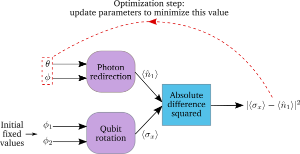
1. The qubit-rotation circuit will contain fixed rotation angles \(\phi_1\) and \(\phi_2\).

2. The photon-redirection circuit will contain two free parameters, the beamsplitter angles \(\theta\) and \(\phi\), which are to be optimized.

3. The outputs of both QNodes will then be fed into the classical node, returning the squared difference of the two quantum functions.

4. Finally, the optimizer will calculate the gradient of the entire computation with respect to the free parameters \(\theta\) and \(\phi\), and update their values.

In essence, we are optimizing the photon-redirection circuit to return the same expectation value as the qubit-rotation circuit, even though they are two completely independent quantum systems.

We can translate this computational graph to the following function, which combines the three nodes into a single hybrid computation. Below, we choose default values \(\phi_1=0.5\), \(\phi_2=0.1\):

def cost(params, phi1=0.5, phi2=0.1):
    """Returns the squared difference between
    the photon-redirection and qubit-rotation QNodes, for
    fixed values of the qubit rotation angles phi1 and phi2"""
    qubit_result = qubit_rotation(phi1, phi2)
    photon_result = photon_redirection(params)
    return squared_difference(qubit_result, photon_result)

Now, we use the built-in GradientDescentOptimizer to perform the optimization for 100 steps. As before, we choose initial beamsplitter parameters of \(\theta=0.01\), \(\phi=0.01\).

# initialise the optimizer
opt = qml.GradientDescentOptimizer(stepsize=0.4)

# set the number of steps
steps = 100
# set the initial parameter values
params = np.array([0.01, 0.01], requires_grad=True)

for i in range(steps):
    # update the circuit parameters
    params = opt.step(cost, params)

    if (i + 1) % 5 == 0:
        print("Cost after step {:5d}: {: .7f}".format(i + 1, cost(params)))

print("Optimized rotation angles: {}".format(params))

Out:

Cost after step     5:  0.2154539
Cost after step    10:  0.0000982
Cost after step    15:  0.0000011
Cost after step    20:  0.0000000
Cost after step    25:  0.0000000
Cost after step    30:  0.0000000
Cost after step    35:  0.0000000
Cost after step    40:  0.0000000
Cost after step    45:  0.0000000
Cost after step    50:  0.0000000
Cost after step    55:  0.0000000
Cost after step    60:  0.0000000
Cost after step    65:  0.0000000
Cost after step    70:  0.0000000
Cost after step    75:  0.0000000
Cost after step    80:  0.0000000
Cost after step    85:  0.0000000
Cost after step    90:  0.0000000
Cost after step    95:  0.0000000
Cost after step   100:  0.0000000
Optimized rotation angles: [1.20671364 0.01      ]

Substituting this into the photon redirection QNode shows that it now produces the same output as the qubit rotation QNode:

result = [1.20671364, 0.01]
print(photon_redirection(result))
print(qubit_rotation(0.5, 0.1))

Out:

0.8731983021146449
0.8731983044562817

This is just a simple example of the kind of hybrid computation that can be carried out in PennyLane. Quantum nodes (bound to different devices) and classical functions can be combined in many different and interesting ways.

About the author

Josh Izaac

Josh is a theoretical physicist, software tinkerer, and occasional baker. At Xanadu, he contributes to the development and growth of Xanadu’s open-source quantum software products.

demos/plugins_hybrid

 

Download Python script

 

Download Notebook

 

View on GitHub