Adjoint Differentiation

Author: Christina Lee. Posted: 23 Nov 2021. Last updated: 23 Nov 2021.

Classical automatic differentiation has two methods of calculation: forward and reverse. The optimal choice of method depends on the structure of the problem; is the function many-to-one or one-to-many? We use the properties of the problem to optimize how we calculate derivatives.

Most methods for calculating the derivatives of quantum circuits are either direct applications of classical gradient methods to quantum simulations, or quantum hardware methods like parameter-shift where we can only extract restricted pieces of information.

Adjoint differentiation straddles these two strategies, taking benefits from each. On simulators, we can examine and modify the state vector at any point. At the same time, we know our quantum circuit holds specific properties not present in an arbitrary classical computation.

Quantum circuits only involve:

1. initialization,

\[|0\rangle,\]

2. application of unitary operators,

\[|\Psi\rangle = U_{n} U_{n-1} \dots U_0 |0\rangle,\]

3. measurement, such as estimating an expectation value of a Hermitian operator,

\[\langle M \rangle = \langle \Psi | M | \Psi \rangle.\]

Since all our operators are unitary, we can easily “undo” or “erase” them by applying their adjoint:

\[U^{\dagger} U | \phi \rangle = |\phi\rangle.\]

The adjoint differentiation method takes advantage of the ability to erase, creating a time- and memory-efficient method for computing quantum gradients on state vector simulators. Tyson Jones and Julien Gacon describe this algorithm in their paper “Efficient calculation of gradients in classical simulations of variational quantum algorithms” .

In this demo, you will learn how adjoint differentiation works and how to request it for your PennyLane QNode. We will also look at the performance benefits.

Time for some code

So how does it work? Instead of jumping straight to the algorithm, let’s explore the above equations and their implementation in a bit more detail.

To start, we import PennyLane and PennyLane’s numpy:

import pennylane as qml
from pennylane import numpy as np

We also need a circuit to simulate:

dev = qml.device('default.qubit', wires=2)

x = np.array([0.1, 0.2, 0.3])

@qml.qnode(dev, diff_method="adjoint")
def circuit(a):
    qml.RX(a[0], wires=0)
    qml.CNOT(wires=(0,1))
    qml.RY(a[1], wires=1)
    qml.RZ(a[2], wires=1)
    return qml.expval(qml.PauliX(wires=1))

The fast c++ simulator device "lightning.qubit" also supports adjoint differentiation, but here we want to quickly prototype a minimal version to illustrate how the algorithm works. We recommend performing adjoint differentiation on "lightning.qubit" for substantial performance increases.

We will use the circuit QNode just for comparison purposes. Throughout this demo, we will instead use a list of its operations ops and a single observable M.

n_gates = 4
n_params = 3

ops = [
    qml.RX(x[0], wires=0),
    qml.CNOT(wires=(0,1)),
    qml.RY(x[1], wires=1),
    qml.RZ(x[2], wires=1)
]
M = qml.PauliX(wires=1)

We create our state by using the "default.qubit" methods _create_basis_state and _apply_operation.

These are private methods that you shouldn’t typically use and are subject to change without a deprecation period, but we use them here to illustrate the algorithm.

Internally, the device uses a 2x2x2x… array to represent the state, whereas the measurement qml.state() and the device attribute dev.state flatten this internal representation.

state = dev._create_basis_state(0)

for op in ops:
    state = dev._apply_operation(state, op)

print(state)

Out:

[[9.82601808e-01-0.14850574j 9.85890302e-02+0.01490027j]
 [7.45635195e-04+0.00493356j 7.43148086e-03-0.04917107j]]

We can think of the expectation \(\langle M \rangle\) as an inner product between a bra and a ket:

\[\langle M \rangle = \langle b | k \rangle = \langle \Psi | M | \Psi \rangle,\]

where

\[\langle b | = \langle \Psi| M = \langle 0 | U_0^{\dagger} \dots U_n^{\dagger} M,\]

\[| k \rangle = |\Psi \rangle = U_n U_{n-1} \dots U_0 |0\rangle.\]

We could have attached \(M\), a Hermitian observable (\(M^{\dagger}=M\)), to either the bra or the ket, but attaching it to the bra side will be useful later.

Using the state calculated above, we can create these \(|b\rangle\) and \(|k\rangle\) vectors.

bra = dev._apply_operation(state, M)
ket = state

Now we use np.vdot to take their inner product. np.vdot sums over all dimensions and takes the complex conjugate of the first input.

M_expval = np.vdot(bra, ket)
print("vdot  : ", M_expval)
print("QNode : ", circuit(x))

Out:

vdot  :  (0.18884787122715616-1.8095277065781732e-19j)
QNode :  0.18884787122715602

We got the same result via both methods! This validates our use of vdot and device methods.

But the dividing line between what makes the “bra” and “ket” vector is actually fairly arbitrary. We can divide the two vectors at any point from one \(\langle 0 |\) to the other \(|0\rangle\). For example, we could have used

\[\langle b_n | = \langle 0 | U_1^{\dagger} \dots U_n^{\dagger} M U_n,\]

\[|k_n \rangle = U_{n-1} \dots U_1 |0\rangle,\]

and gotten the exact same results. Here, the subscript \(n\) is used to indicate that \(U_n\) was moved to the bra side of the expression. Let’s calculate that instead:

bra_n = dev._create_basis_state(0)

for op in ops:
    bra_n = dev._apply_operation(bra_n, op)
bra_n = dev._apply_operation(bra_n, M)
bra_n = dev._apply_operation(bra_n, qml.adjoint(ops[-1]))

ket_n = dev._create_basis_state(0)

for op in ops[:-1]: # don't apply last operation
    ket_n = dev._apply_operation(ket_n, op)

M_expval_n = np.vdot(bra_n, ket_n)
print(M_expval_n)

Out:

(0.18884787122715616+5.248486695784019e-19j)

Same answer!

We can calculate this in a more efficient way if we already have the initial state \(| \Psi \rangle\). To shift the splitting point, we don’t have to recalculate everything from scratch. We just remove the operation from the ket and add it to the bra:

\[\langle b_n | = \langle b | U_n,\]

\[|k_n\rangle = U_n^{\dagger} |k\rangle .\]

For the ket vector, you can think of \(U_n^{\dagger}\) as “eating” its corresponding unitary from the vector, erasing it from the list of operations.

Of course, we actually work with the conjugate transpose of \(\langle b_n |\),

\[|b_n\rangle = U_n^{\dagger} | b \rangle.\]

Once we write it in this form, we see that the adjoint of the operation \(U_n^{\dagger}\) operates on both \(|k_n\rangle\) and \(|b_n\rangle\) to move the splitting point right.

Let’s call this the “version 2” method.

bra_n_v2 = dev._apply_operation(state, M)
ket_n_v2 = state

adj_op = qml.adjoint(ops[-1])

bra_n_v2 = dev._apply_operation(bra_n_v2, adj_op)
ket_n_v2 = dev._apply_operation(ket_n_v2, adj_op)

M_expval_n_v2 = np.vdot(bra_n_v2, ket_n_v2)
print(M_expval_n_v2)

Out:

(0.18884787122715613-9.998596039908862e-20j)

Much simpler!

We can easily iterate over all the operations to show that the same result occurs no matter where you split the operations:

\[\langle b_i | = \langle b_{i+1}| U_{i},\]

\[|k_{i+1} \rangle = U_{i} |k_{i}\rangle.\]

Rewritten, we have our iteration formulas

\[| b_i \rangle = U_i^{\dagger} |b_{i+1}\rangle,\]

\[| k_i \rangle = U_i^{\dagger} |k_{i+1}\rangle.\]

For each iteration, we move an operation from the ket side to the bra side. We start near the center at \(U_n\) and reverse through the operations list until we reach \(U_0\).

bra_loop = dev._apply_operation(state, M)
ket_loop = state

for op in reversed(ops):
    adj_op = qml.adjoint(op)
    bra_loop = dev._apply_operation(bra_loop, adj_op)
    ket_loop = dev._apply_operation(ket_loop, adj_op)
    print(np.vdot(bra_loop, ket_loop))

Out:

(0.18884787122715613-9.998596039908862e-20j)
(0.18884787122715607-1.7961676396687185e-20j)
(0.18884787122715607-1.7961676396687185e-20j)
(0.1888478712271561-1.7961676396687185e-20j)

Finally to Derivatives!

We showed how to calculate the same thing a bunch of different ways. Why is this useful? Wherever we cut, we can stick additional things in the middle. What are we sticking in the middle? The derivative of a gate.

For simplicity’s sake, assume each unitary operation \(U_i\) is a function of a single parameter \(\theta_i\). For non-parametrized gates like CNOT, we say its derivative is zero. We can also generalize the algorithm to multi-parameter gates, but we leave those out for now.

Remember that each parameter occurs twice in \(\langle M \rangle\): once in the bra and once in the ket. Therefore, we use the product rule to take the derivative with respect to both locations:

\[\frac{\partial \langle M \rangle}{\partial \theta_i} = \langle 0 | U_1^{\dagger} \dots \frac{\text{d} U_i^{\dagger}}{\text{d} \theta_i} \dots M \dots U_i \dots U_1 | 0\rangle.\]

\[+ \langle 0 | U_1^{\dagger} \dots U_i^{\dagger} \dots M \dots \frac{\text{d} U_i}{\text{d} \theta_i} \dots U_1 |0\rangle\]

We can now notice that those two components are complex conjugates of each other, so we can further simplify. Note that each term is not an expectation value of a Hermitian observable, and therefore not guaranteed to be real. When we add them together, the imaginary part cancels out, and we obtain twice the value of the real part:

\[= 2 \cdot \text{Re}\left( \langle 0 | U_1^{\dagger} \dots U_i^{\dagger} \dots M \dots \frac{\text{d} U_i}{\text{d} \theta_i} \dots U_1 |0\rangle \right).\]

We can take that formula and break it into its “bra” and “ket” halves for a derivative at the \(i\) th position:

\[\frac{\partial \langle M \rangle }{\partial \theta_i } = 2 \text{Re} \left( \langle b_i | \frac{\text{d} U_i }{\text{d} \theta_i} | k_i \rangle \right)\]

where

\[\langle b_i | = \langle 0 | U_1^{\dagger} \dots U_n^{\dagger} M U_n \dots U_{i+1},\]

\[|k_i \rangle = U_{i-1} \dots U_1 |0\rangle.\]

Notice that \(U_i\) does not appear in either the bra or the ket in the above equations. These formulas differ from the ones we used when just calculating the expectation value. For the actual derivative calculation, we use a temporary version of the bra,

\[| \tilde{k}_i \rangle = \frac{\text{d} U_i}{\text{d} \theta_i} | k_i \rangle\]

and use these to get the derivative

\[\frac{\partial \langle M \rangle}{\partial \theta_i} = 2 \text{Re}\left( \langle b_i | \tilde{k}_i \rangle \right).\]

Both the bra and the ket can be calculated recursively:

\[| b_{i} \rangle = U^{\dagger}_{i+1} |b_{i+1}\rangle,\]

\[| k_{i} \rangle = U^{\dagger}_{i} |k_{i+1}\rangle.\]

We can iterate through the operations starting at \(n\) and ending at \(1\).

We do have to calculate initial state first, the “forward” pass:

\[|\Psi\rangle = U_{n} U_{n-1} \dots U_0 |0\rangle.\]

Once we have that, we only have about the same amount of work to calculate all the derivatives, instead of quadratically more work.

Derivative of an Operator

One final thing before we get back to coding: how do we get the derivative of an operator?

Most parametrized gates can be represented in terms of Pauli Rotations, which can be written as

\[U = e^{i c \hat{G} \theta}\]

for a Pauli matrix \(\hat{G}\), a constant \(c\), and the parameter \(\theta\). Thus we can easily calculate their derivatives:

\[\frac{\text{d} U}{\text{d} \theta} = i c \hat{G} e^{i c \hat{G} \theta} = i c \hat{G} U .\]

Luckily, PennyLane already has a built-in function for calculating this.

grad_op0 = qml.operation.operation_derivative(ops[0])
print(grad_op0)

Out:

[[-0.02498958+0.j          0.        -0.49937513j]
 [ 0.        -0.49937513j -0.02498958+0.j        ]]

Now for calculating the full derivative using the adjoint method!

We loop over the reversed operations, just as before. But if the operation has a parameter, we calculate its derivative and append it to a list before moving on. Since the operation_derivative function spits back out a matrix instead of an operation, we have to use dev._apply_unitary instead to create \(|\tilde{k}_i\rangle\).

bra = dev._apply_operation(state, M)
ket = state

grads = []

for op in reversed(ops):
    adj_op = qml.adjoint(op)
    ket = dev._apply_operation(ket, adj_op)

    # Calculating the derivative
    if op.num_params != 0:
        dU = qml.operation.operation_derivative(op)

        ket_temp = dev._apply_unitary(ket, dU, op.wires)

        dM = 2 * np.real(np.vdot(bra, ket_temp))
        grads.append(dM)

    bra = dev._apply_operation(bra, adj_op)


# Finally reverse the order of the gradients
# since we calculated them in reverse
grads = grads[::-1]

print("our calculation: ", grads)

grad_compare = qml.grad(circuit)(x)
print("comparison: ", grad_compare)

Out:

our calculation:  [-0.0189479892336121, 0.9316157966884504, -0.05841749223216956]
comparison:  [-0.01894799  0.9316158  -0.05841749]

It matches!!!

If you want to use adjoint differentiation without having to code up your own method that can support arbitrary circuits, you can use diff_method="adjoint" in PennyLane with "default.qubit" or PennyLane’s fast C++ simulator "lightning.qubit".

dev_lightning = qml.device('lightning.qubit', wires=2)

@qml.qnode(dev_lightning, diff_method="adjoint")
def circuit_adjoint(a):
    qml.RX(a[0], wires=0)
    qml.CNOT(wires=(0,1))
    qml.RY(a[1], wires=1)
    qml.RZ(a[2], wires=1)
    return qml.expval(M)

print(qml.grad(circuit_adjoint)(x))

Out:

[-0.01894799  0.9316158  -0.05841749]

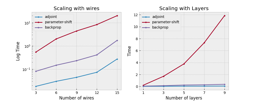
Performance

The algorithm gives us the correct answers, but is it worth using? Parameter-shift gradients require at least two executions per parameter, so that method gets more and more expensive with the size of the circuit, especially on simulators. Backpropagation demonstrates decent time scaling, but requires more and more memory as the circuit gets larger. Simulation of large circuits is already RAM-limited, and backpropagation constrains the size of possible circuits even more. PennyLane also achieves backpropagation derivatives from a Python simulator and interface-specific functions. The "lightning.qubit" device does not support backpropagation, so backpropagation derivatives lose the speedup from an optimized simulator.

With adjoint differentiation on "lightning.qubit", you can get the best of both worlds: fast and memory efficient.

But how fast? The provided script here generated the following images on a mid-range laptop. The backpropagation times were produced with the Python simulator "default.qubit", while parameter-shift and adjoint differentiation times were calculated with "lightning.qubit". The adjoint method clearly wins out for performance.

Conclusions

So what have we learned? Adjoint differentiation is an efficient method for differentiating quantum circuits with state vector simulation. It scales nicely in time without excessive memory requirements. Now that you’ve seen how the algorithm works, you can better understand what is happening when you select adjoint differentiation from one of PennyLane’s simulators.

Bibliography

Jones and Gacon. Efficient calculation of gradients in classical simulations of variational quantum algorithms. https://arxiv.org/abs/2009.02823

Xiu-Zhe Luo, Jin-Guo Liu, Pan Zhang, and Lei Wang. Yao.jl: Extensible, efficient framework for quantum algorithm design , 2019

About the author

Christina Lee

Christina is currently a quantum software developer at Xanadu working on PennyLane. Outside of coding, she enjoys running, yoga, and piano.

demos/tutorial_adjoint_diff

 

Download Python script

 

Download Notebook

 

View on GitHub