Basic tutorial: qubit rotation

Author: Josh Izaac — Posted: 11 October 2019. Last updated: 19 January 2021.

To see how PennyLane allows the easy construction and optimization of quantum functions, let’s consider the simple case of qubit rotation the PennyLane version of the ‘Hello, world!’ example.

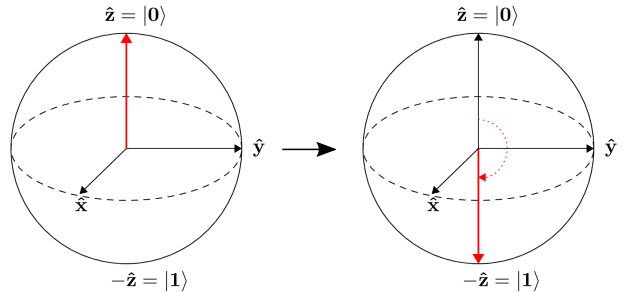
The task at hand is to optimize two rotation gates in order to flip a single qubit from state \(\left|0\right\rangle\) to state \(\left|1\right\rangle\).

The quantum circuit

In the qubit rotation example, we wish to implement the following quantum circuit:

Breaking this down step-by-step, we first start with a qubit in the ground state \(|0\rangle = \begin{bmatrix}1 & 0 \end{bmatrix}^T\), and rotate it around the x-axis by applying the gate

\[\begin{split}R_x(\phi_1) = e^{-i \phi_1 \sigma_x /2} = \begin{bmatrix} \cos \frac{\phi_1}{2} & -i \sin \frac{\phi_1}{2} \\ -i \sin \frac{\phi_1}{2} & \cos \frac{\phi_1}{2} \end{bmatrix},\end{split}\]

and then around the y-axis via the gate

\[\begin{split}R_y(\phi_2) = e^{-i \phi_2 \sigma_y/2} = \begin{bmatrix} \cos \frac{\phi_2}{2} & - \sin \frac{\phi_2}{2} \\ \sin \frac{\phi_2}{2} & \cos \frac{\phi_2}{2} \end{bmatrix}.\end{split}\]

After these operations the qubit is now in the state

\[| \psi \rangle = R_y(\phi_2) R_x(\phi_1) | 0 \rangle.\]

Finally, we measure the expectation value \(\langle \psi \mid \sigma_z \mid \psi \rangle\) of the Pauli-Z operator

\[\begin{split}\sigma_z = \begin{bmatrix} 1 & 0 \\ 0 & -1 \end{bmatrix}.\end{split}\]

Using the above to calculate the exact expectation value, we find that

\[\langle \psi \mid \sigma_z \mid \psi \rangle = \langle 0 \mid R_x(\phi_1)^\dagger R_y(\phi_2)^\dagger \sigma_z R_y(\phi_2) R_x(\phi_1) \mid 0 \rangle = \cos(\phi_1)\cos(\phi_2).\]

Depending on the circuit parameters \(\phi_1\) and \(\phi_2\), the output expectation lies between \(1\) (if \(\left|\psi\right\rangle = \left|0\right\rangle\)) and \(-1\) (if \(\left|\psi\right\rangle = \left|1\right\rangle\)).

Let’s see how we can easily implement and optimize this circuit using PennyLane.

Importing PennyLane and NumPy

The first thing we need to do is import PennyLane, as well as the wrapped version of NumPy provided by PennyLane.

import pennylane as qml
from pennylane import numpy as np

Important

When constructing a hybrid quantum/classical computational model with PennyLane, it is important to always import NumPy from PennyLane, not the standard NumPy!

By importing the wrapped version of NumPy provided by PennyLane, you can combine the power of NumPy with PennyLane:

• continue to use the classical NumPy functions and arrays you know and love

• combine quantum functions (evaluated on quantum hardware/simulators) and classical functions (provided by NumPy)

• allow PennyLane to automatically calculate gradients of both classical and quantum functions

Creating a device

Before we can construct our quantum node, we need to initialize a device.

Definition

Any computational object that can apply quantum operations and return a measurement value is called a quantum device.

In PennyLane, a device could be a hardware device (such as the IBM QX4, via the PennyLane-PQ plugin), or a software simulator (such as Strawberry Fields, via the PennyLane-SF plugin).

Tip

Devices are loaded in PennyLane via the function device()

PennyLane supports devices using both the qubit model of quantum computation and devices using the CV model of quantum computation. In fact, even a hybrid computation containing both qubit and CV quantum nodes is possible; see the hybrid computation example for more details.

For this tutorial, we are using the qubit model, so let’s initialize the 'default.qubit' device provided by PennyLane; a simple pure-state qubit simulator.

dev1 = qml.device("default.qubit", wires=1)

For all devices, device() accepts the following arguments:

• name: the name of the device to be loaded

• wires: the number of subsystems to initialize the device with

Here, as we only require a single qubit for this example, we set wires=1.

Constructing the QNode

Now that we have initialized our device, we can begin to construct a quantum node (or QNode).

Definition

QNodes are an abstract encapsulation of a quantum function, described by a quantum circuit. QNodes are bound to a particular quantum device, which is used to evaluate expectation and variance values of this circuit.

Tip

QNodes can be constructed via the QNode class, or by using the provided qnode() decorator.

First, we need to define the quantum function that will be evaluated in the QNode:

def circuit(params):
    qml.RX(params[0], wires=0)
    qml.RY(params[1], wires=0)
    return qml.expval(qml.PauliZ(0))

This is a simple circuit, matching the one described above. Notice that the function circuit() is constructed as if it were any other Python function; it accepts a positional argument params, which may be a list, tuple, or array, and uses the individual elements for gate parameters.

However, quantum functions are a restricted subset of Python functions. For a Python function to also be a valid quantum function, there are some important restrictions:

• Quantum functions must contain quantum operations, one operation per line, in the order in which they are to be applied.

  In addition, we must always specify the subsystem the operation applies to, by passing the wires argument; this may be a list or an integer, depending on how many wires the operation acts on.

  For a full list of quantum operations, see the documentation.

• Quantum functions must return either a single or a tuple of measured observables.

  As a result, the quantum function always returns a classical quantity, allowing the QNode to interface with other classical functions (and also other QNodes).

  For a full list of observables, see the documentation. The documentation also provides details on supported measurement return types.

Note

Certain devices may only support a subset of the available PennyLane operations/observables, or may even provide additional operations/observables. Please consult the documentation for the plugin/device for more details.

Once we have written the quantum function, we convert it into a QNode running on device dev1 by applying the qnode() decorator. directly above the function definition:

@qml.qnode(dev1, interface="autograd")
def circuit(params):
    qml.RX(params[0], wires=0)
    qml.RY(params[1], wires=0)
    return qml.expval(qml.PauliZ(0))

Thus, our circuit() quantum function is now a QNode, which will run on device dev1 every time it is evaluated.

To evaluate, we simply call the function with some appropriate numerical inputs:

print(circuit([0.54, 0.12]))

Out:

0.8515405859048369

Calculating quantum gradients

The gradient of the function circuit, encapsulated within the QNode, can be evaluated by utilizing the same quantum device (dev1) that we used to evaluate the function itself.

PennyLane incorporates both analytic differentiation, as well as numerical methods (such as the method of finite differences). Both of these are done automatically.

We can differentiate by using the built-in grad() function. This returns another function, representing the gradient (i.e., the vector of partial derivatives) of circuit. The gradient can be evaluated in the same way as the original function:

dcircuit = qml.grad(circuit, argnum=0)

The function grad() itself returns a function, representing the derivative of the QNode with respect to the argument specified in argnum. In this case, the function circuit takes one argument (params), so we specify argnum=0. Because the argument has two elements, the returned gradient is two-dimensional. We can then evaluate this gradient function at any point in the parameter space.

print(dcircuit([0.54, 0.12]))

Out:

[array(-0.51043865), array(-0.1026782)]

A note on arguments

Quantum circuit functions, being a restricted subset of Python functions, can also make use of multiple positional arguments and keyword arguments. For example, we could have defined the above quantum circuit function using two positional arguments, instead of one array argument:

@qml.qnode(dev1, interface="autograd")
def circuit2(phi1, phi2):
    qml.RX(phi1, wires=0)
    qml.RY(phi2, wires=0)
    return qml.expval(qml.PauliZ(0))

When we calculate the gradient for such a function, the usage of argnum will be slightly different. In this case, argnum=0 will return the gradient with respect to only the first parameter (phi1), and argnum=1 will give the gradient for phi2. To get the gradient with respect to both parameters, we can use argnum=[0,1]:

dcircuit = qml.grad(circuit2, argnum=[0, 1])
print(dcircuit(0.54, 0.12))

Out:

(array(-0.51043865), array(-0.1026782))

Keyword arguments may also be used in your custom quantum function. PennyLane does not differentiate QNodes with respect to keyword arguments, so they are useful for passing external data to your QNode.

Optimization

Definition

If using the default NumPy/Autograd interface, PennyLane provides a collection of optimizers based on gradient descent. These optimizers accept a cost function and initial parameters, and utilize PennyLane’s automatic differentiation to perform gradient descent.

Tip

See introduction/optimizers for details and documentation of available optimizers

Next, let’s make use of PennyLane’s built-in optimizers to optimize the two circuit parameters \(\phi_1\) and \(\phi_2\) such that the qubit, originally in state \(\left|0\right\rangle\), is rotated to be in state \(\left|1\right\rangle\). This is equivalent to measuring a Pauli-Z expectation value of \(-1\), since the state \(\left|1\right\rangle\) is an eigenvector of the Pauli-Z matrix with eigenvalue \(\lambda=-1\).

In other words, the optimization procedure will find the weights \(\phi_1\) and \(\phi_2\) that result in the following rotation on the Bloch sphere:

To do so, we need to define a cost function. By minimizing the cost function, the optimizer will determine the values of the circuit parameters that produce the desired outcome.

In this case, our desired outcome is a Pauli-Z expectation value of \(-1\). Since we know that the Pauli-Z expectation is bound between \([-1, 1]\), we can define our cost directly as the output of the QNode:

def cost(x):
    return circuit(x)

To begin our optimization, let’s choose small initial values of \(\phi_1\) and \(\phi_2\):

init_params = np.array([0.011, 0.012], requires_grad=True)
print(cost(init_params))

Out:

0.9998675058299391

We can see that, for these initial parameter values, the cost function is close to \(1\).

Finally, we use an optimizer to update the circuit parameters for 100 steps. We can use the built-in GradientDescentOptimizer class:

# initialise the optimizer
opt = qml.GradientDescentOptimizer(stepsize=0.4)

# set the number of steps
steps = 100
# set the initial parameter values
params = init_params

for i in range(steps):
    # update the circuit parameters
    params = opt.step(cost, params)

    if (i + 1) % 5 == 0:
        print("Cost after step {:5d}: {: .7f}".format(i + 1, cost(params)))

print("Optimized rotation angles: {}".format(params))

Out:

Cost after step     5:  0.9961778
Cost after step    10:  0.8974944
Cost after step    15:  0.1440490
Cost after step    20: -0.1536720
Cost after step    25: -0.9152496
Cost after step    30: -0.9994046
Cost after step    35: -0.9999964
Cost after step    40: -1.0000000
Cost after step    45: -1.0000000
Cost after step    50: -1.0000000
Cost after step    55: -1.0000000
Cost after step    60: -1.0000000
Cost after step    65: -1.0000000
Cost after step    70: -1.0000000
Cost after step    75: -1.0000000
Cost after step    80: -1.0000000
Cost after step    85: -1.0000000
Cost after step    90: -1.0000000
Cost after step    95: -1.0000000
Cost after step   100: -1.0000000
Optimized rotation angles: [7.15266381e-18 3.14159265e+00]

We can see that the optimization converges after approximately 40 steps.

Substituting this into the theoretical result \(\langle \psi \mid \sigma_z \mid \psi \rangle = \cos\phi_1\cos\phi_2\), we can verify that this is indeed one possible value of the circuit parameters that produces \(\langle \psi \mid \sigma_z \mid \psi \rangle=-1\), resulting in the qubit being rotated to the state \(\left|1\right\rangle\).

Note

Some optimizers, such as AdagradOptimizer, have internal hyperparameters that are stored in the optimizer instance. These can be reset using the reset() method.

Continue on to the next tutorial, Gaussian transformation, to see a similar example using continuous-variable (CV) quantum nodes.

About the author

Josh Izaac

Josh is a theoretical physicist, software tinkerer, and occasional baker. At Xanadu, he contributes to the development and growth of Xanadu’s open-source quantum software products.

demos/tutorial_qubit_rotation

 

Download Python script

 

Download Notebook

 

View on GitHub