Quantum gradients with backpropagation

Author: Josh Izaac — Posted: 11 August 2020. Last updated: 31 January 2021.

In PennyLane, any quantum device, whether a hardware device or a simulator, can be trained using the parameter-shift rule to compute quantum gradients. Indeed, the parameter-shift rule is ideally suited to hardware devices, as it does not require any knowledge about the internal workings of the device; it is sufficient to treat the device as a ‘black box’, and to query it with different input values in order to determine the gradient.

When working with simulators, however, we do have access to the internal (classical) computations being performed. This allows us to take advantage of other methods of computing the gradient, such as backpropagation, which may be advantageous in certain regimes. In this tutorial, we will compare and contrast the parameter-shift rule against backpropagation, using the PennyLane default.qubit device.

The parameter-shift rule

The parameter-shift rule states that, given a variational quantum circuit \(U(\boldsymbol \theta)\) composed of parametrized Pauli rotations, and some measured observable \(\hat{B}\), the derivative of the expectation value

\[\langle \hat{B} \rangle (\boldsymbol\theta) = \langle 0 \vert U(\boldsymbol\theta)^\dagger \hat{B} U(\boldsymbol\theta) \vert 0\rangle\]

with respect to the input circuit parameters \(\boldsymbol{\theta}\) is given by

\[\nabla_{\theta_i}\langle \hat{B} \rangle(\boldsymbol\theta) = \frac{1}{2} \left[ \langle \hat{B} \rangle\left(\boldsymbol\theta + \frac{\pi}{2}\hat{\mathbf{e}}_i\right) - \langle \hat{B} \rangle\left(\boldsymbol\theta - \frac{\pi}{2}\hat{\mathbf{e}}_i\right) \right].\]

Thus, the gradient of the expectation value can be calculated by evaluating the same variational quantum circuit, but with shifted parameter values (hence the name, parameter-shift rule!).

Let’s have a go implementing the parameter-shift rule manually in PennyLane.

import pennylane as qml
from pennylane import numpy as np
from matplotlib import pyplot as plt

# set the random seed
np.random.seed(42)

# create a device to execute the circuit on
dev = qml.device("default.qubit", wires=3)

@qml.qnode(dev, diff_method="parameter-shift", interface="autograd")
def circuit(params):
    qml.RX(params[0], wires=0)
    qml.RY(params[1], wires=1)
    qml.RZ(params[2], wires=2)

    qml.broadcast(qml.CNOT, wires=[0, 1, 2], pattern="ring")

    qml.RX(params[3], wires=0)
    qml.RY(params[4], wires=1)
    qml.RZ(params[5], wires=2)

    qml.broadcast(qml.CNOT, wires=[0, 1, 2], pattern="ring")
    return qml.expval(qml.PauliY(0) @ qml.PauliZ(2))

Let’s test the variational circuit evaluation with some parameter input:

# initial parameters
params = np.random.random([6], requires_grad=True)

print("Parameters:", params)
print("Expectation value:", circuit(params))

Out:

Parameters: [0.37454012 0.95071431 0.73199394 0.59865848 0.15601864 0.15599452]
Expectation value: -0.11971365706871569

We can also draw the executed quantum circuit:

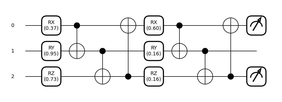
fig, ax = qml.draw_mpl(circuit, decimals=2)(params)
plt.show()

Now that we have defined our variational circuit QNode, we can construct a function that computes the gradient of the \(i\text{th}\) parameter using the parameter-shift rule.

def parameter_shift_term(qnode, params, i):
    shifted = params.copy()
    shifted[i] += np.pi/2
    forward = qnode(shifted)  # forward evaluation

    shifted[i] -= np.pi
    backward = qnode(shifted) # backward evaluation

    return 0.5 * (forward - backward)

# gradient with respect to the first parameter
print(parameter_shift_term(circuit, params, 0))

Out:

-0.0651887722495812

In order to compute the gradient with respect to all parameters, we need to loop over the index i:

def parameter_shift(qnode, params):
    gradients = np.zeros([len(params)])

    for i in range(len(params)):
        gradients[i] = parameter_shift_term(qnode, params, i)

    return gradients

print(parameter_shift(circuit, params))

Out:

[-6.51887722e-02 -2.72891905e-02 -2.77555756e-17 -9.33934621e-02
 -7.61067572e-01  0.00000000e+00]

We can compare this to PennyLane’s built-in quantum gradient support by using the qml.grad function, which allows us to compute gradients of hybrid quantum-classical cost functions. Remember, when we defined the QNode, we specified that we wanted it to be differentiable using the parameter-shift method (diff_method="parameter-shift").

grad_function = qml.grad(circuit)
print(grad_function(params)[0])

Out:

-0.06518877224958117

Alternatively, we can directly compute quantum gradients of QNodes using PennyLane’s built in qml.gradients module:

print(qml.gradients.param_shift(circuit)(params))

Out:

(array(-0.06518877), array(-0.02728919), array(-4.10464615e-17), array(-0.09339346), array(-0.76106757), array(5.86901964e-19))

If you count the number of quantum evaluations, you will notice that we had to evaluate the circuit 2*len(params) number of times in order to compute the quantum gradient with respect to all parameters. While reasonably fast for a small number of parameters, as the number of parameters in our quantum circuit grows, so does both

1. the circuit depth (and thus the time taken to evaluate each expectation value or ‘forward’ pass), and

2. the number of parameter-shift evaluations required.

Both of these factors increase the time taken to compute the gradient with respect to all parameters.

Benchmarking

Let’s consider an example with a significantly larger number of parameters. We’ll make use of the StronglyEntanglingLayers template to make a more complicated QNode.

dev = qml.device("default.qubit", wires=4)

@qml.qnode(dev, diff_method="parameter-shift", interface="autograd")
def circuit(params):
    qml.StronglyEntanglingLayers(params, wires=[0, 1, 2, 3])
    return qml.expval(qml.PauliZ(0) @ qml.PauliZ(1) @ qml.PauliZ(2) @ qml.PauliZ(3))

# initialize circuit parameters
param_shape = qml.StronglyEntanglingLayers.shape(n_wires=4, n_layers=15)
params = np.random.normal(scale=0.1, size=param_shape, requires_grad=True)
print(params.size)
print(circuit(params))

Out:

180
0.8947771876917714

This circuit has 180 parameters. Let’s see how long it takes to perform a forward pass of the circuit.

import timeit

reps = 3
num = 10
times = timeit.repeat("circuit(params)", globals=globals(), number=num, repeat=reps)
forward_time = min(times) / num

print(f"Forward pass (best of {reps}): {forward_time} sec per loop")

Out:

Forward pass (best of 3): 0.021240537099993163 sec per loop

We can now estimate the time taken to compute the full gradient vector, and see how this compares.

# create the gradient function
grad_fn = qml.grad(circuit)

times = timeit.repeat("grad_fn(params)", globals=globals(), number=num, repeat=reps)
backward_time = min(times) / num

print(f"Gradient computation (best of {reps}): {backward_time} sec per loop")

Out:

Gradient computation (best of 3): 9.981895925499998 sec per loop

Based on the parameter-shift rule, we expect that the amount of time to compute the quantum gradients should be approximately \(2p\Delta t_{f}\) where \(p\) is the number of parameters and \(\Delta t_{f}\) if the time taken for the forward pass. Let’s verify this:

print(2 * forward_time * params.size)

Out:

7.646593355997539

Backpropagation

An alternative to the parameter-shift rule for computing gradients is reverse-mode autodifferentiation. Unlike the parameter-shift method, which requires \(2p\) circuit evaluations for \(p\) parameters, reverse-mode requires only a single forward pass of the differentiable function to compute the gradient of all variables, at the expense of increased memory usage. During the forward pass, the results of all intermediate subexpressions are stored; the computation is then traversed in reverse, with the gradient computed by repeatedly applying the chain rule. In most classical machine learning settings (where we are training scalar loss functions consisting of a large number of parameters), reverse-mode autodifferentiation is the preferred method of autodifferentiation—the reduction in computational time enables larger and more complex models to be successfully trained. The backpropagation algorithm is a particular special-case of reverse-mode autodifferentiation, which has helped lead to the machine learning explosion we see today.

In quantum machine learning, however, the inability to store and utilize the results of intermediate quantum operations on hardware remains a barrier to using backprop; while reverse-mode autodifferentiation works fine for small quantum simulations, only the parameter-shift rule can be used to compute gradients on quantum hardware directly. Nevertheless, when training quantum models via classical simulation, it’s useful to explore the regimes where reverse-mode differentiation may be a better choice than the parameter-shift rule.

Benchmarking

When creating a QNode, PennyLane supports various methods of differentiation, including "parameter-shift" (which we used previously), "finite-diff", "reversible", and "backprop". While "parameter-shift" works with all devices (simulator or hardware), "backprop" will only work for specific simulator devices that are designed to support backpropagation.

One such device is default.qubit. It has backends written using TensorFlow, JAX, and Autograd, so when used with the TensorFlow, JAX, and Autograd interfaces respectively, supports backpropagation. In this demo, we will use the default Autograd interface.

dev = qml.device("default.qubit", wires=4)

When defining the QNode, we specify diff_method="backprop" to ensure that we are using backpropagation mode. Note that this is the default differentiation mode for the default.qubit device.

@qml.qnode(dev, diff_method="backprop", interface="autograd")
def circuit(params):
    qml.StronglyEntanglingLayers(params, wires=[0, 1, 2, 3])
    return qml.expval(qml.PauliZ(0) @ qml.PauliZ(1) @ qml.PauliZ(2) @ qml.PauliZ(3))

# initialize circuit parameters
param_shape = qml.StronglyEntanglingLayers.shape(n_wires=4, n_layers=15)
params = np.random.normal(scale=0.1, size=param_shape, requires_grad=True)
print(circuit(params))

Out:

0.9358535378025545

Let’s see how long it takes to perform a forward pass of the circuit.

import timeit

reps = 3
num = 10
times = timeit.repeat("circuit(params)", globals=globals(), number=num, repeat=reps)
forward_time = min(times) / num
print(f"Forward pass (best of {reps}): {forward_time} sec per loop")

Out:

Forward pass (best of 3): 0.0580262330000096 sec per loop

Comparing this to the forward pass from default.qubit, we note that there is some potential overhead from using backpropagation. We can now estimate the time required to perform a gradient computation via backpropagation:

times = timeit.repeat("qml.grad(circuit)(params)", globals=globals(), number=num, repeat=reps)
backward_time = min(times) / num
print(f"Backward pass (best of {reps}): {backward_time} sec per loop")

Out:

Backward pass (best of 3): 0.1668012636000185 sec per loop

Unlike with the parameter-shift rule, the time taken to perform the backwards pass appears of the order of a single forward pass! This can significantly speed up training of simulated circuits with many parameters.

Time comparison

Let’s compare the two differentiation approaches as the number of trainable parameters in the variational circuit increases, by timing both the forward pass and the gradient computation as the number of layers is allowed to increase.

dev = qml.device("default.qubit", wires=4)

def circuit(params):
    qml.StronglyEntanglingLayers(params, wires=[0, 1, 2, 3])
    return qml.expval(qml.PauliZ(0) @ qml.PauliZ(1) @ qml.PauliZ(2) @ qml.PauliZ(3))

We’ll continue to use the same ansatz as before, but to reduce the time taken to collect the data, we’ll reduce the number and repetitions of timings per data point. Below, we loop over a variational circuit depth ranging from 0 (no gates/ trainable parameters) to 20. Each layer will contain \(3N\) parameters, where \(N\) is the number of wires (in this case, we have \(N=4\)).

reps = 2
num = 3

forward_shift = []
gradient_shift = []
forward_backprop = []
gradient_backprop = []

for depth in range(0, 21):
    param_shape = qml.StronglyEntanglingLayers.shape(n_wires=4, n_layers=depth)
    params = np.random.normal(scale=0.1, size=param_shape, requires_grad=True)
    num_params = params.size

    # forward pass timing
    # ===================

    qnode_shift = qml.QNode(circuit, dev, diff_method="parameter-shift", interface="autograd")
    qnode_backprop = qml.QNode(circuit, dev, diff_method="backprop", interface="autograd")

    # parameter-shift
    t = timeit.repeat("qnode_shift(params)", globals=globals(), number=num, repeat=reps)
    forward_shift.append([num_params, min(t) / num])

    # backprop
    t = timeit.repeat("qnode_backprop(params)", globals=globals(), number=num, repeat=reps)
    forward_backprop.append([num_params, min(t) / num])

    if num_params == 0:
        continue

    # Gradient timing
    # ===============

    qnode_shift = qml.QNode(circuit, dev, diff_method="parameter-shift", interface="autograd")
    qnode_backprop = qml.QNode(circuit, dev, diff_method="backprop", interface="autograd")

    # parameter-shift
    t = timeit.repeat("qml.grad(qnode_shift)(params)", globals=globals(), number=num, repeat=reps)
    gradient_shift.append([num_params, min(t) / num])

    # backprop
    t = timeit.repeat("qml.grad(qnode_backprop)(params)", globals=globals(), number=num, repeat=reps)
    gradient_backprop.append([num_params, min(t) / num])

gradient_shift = np.array(gradient_shift).T
gradient_backprop = np.array(gradient_backprop).T
forward_shift = np.array(forward_shift).T
forward_backprop = np.array(forward_backprop).T

We now import matplotlib, and plot the results.

plt.style.use("bmh")

fig, ax = plt.subplots(1, 1, figsize=(6, 4))

ax.plot(*gradient_shift, '.-', label="Parameter-shift")
ax.plot(*gradient_backprop, '.-', label="Backprop")
ax.set_ylabel("Time (s)")
ax.set_xlabel("Number of parameters")
ax.legend()

plt.show()

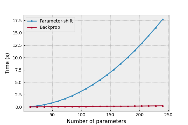
We can see that the computational time for the parameter-shift rule increases with increasing number of parameters, as expected, whereas the computational time for backpropagation appears much more constant, with perhaps a minute linear increase with \(p\). Note that the plots are not perfectly linear, with some ‘bumpiness’ or noisiness. This is likely due to low-level operating system jitter, and other environmental fluctuations—increasing the number of repeats can help smooth out the plot.

For a better comparison, we can scale the time required for computing the quantum gradients against the time taken for the corresponding forward pass:

gradient_shift[1] /= forward_shift[1, 1:]
gradient_backprop[1] /= forward_backprop[1, 1:]

fig, ax = plt.subplots(1, 1, figsize=(6, 4))

ax.plot(*gradient_shift, '.-', label="Parameter-shift")
ax.plot(*gradient_backprop, '.-', label="Backprop")

# perform a least squares regression to determine the linear best fit/gradient
# for the normalized time vs. number of parameters
x = gradient_shift[0]
m_shift, c_shift = np.polyfit(*gradient_shift, deg=1)
m_back, c_back = np.polyfit(*gradient_backprop, deg=1)

ax.plot(x, m_shift * x + c_shift, '--', label=f"{m_shift:.2f}p{c_shift:+.2f}")
ax.plot(x, m_back * x + c_back, '--', label=f"{m_back:.2f}p{c_back:+.2f}")

ax.set_ylabel("Normalized time")
ax.set_xlabel("Number of parameters")
ax.set_xscale("log")
ax.set_yscale("log")
ax.legend()

plt.show()

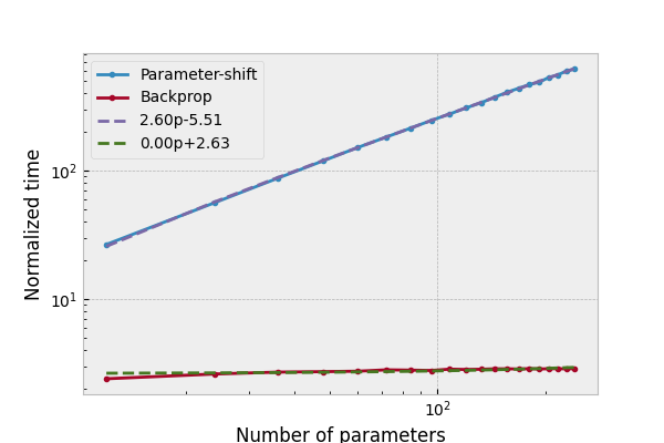
We can now see clearly that there is constant overhead for backpropagation with default.qubit, but the parameter-shift rule scales as \(\sim 2p\).

About the author

Josh Izaac

Josh is a theoretical physicist, software tinkerer, and occasional baker. At Xanadu, he contributes to the development and growth of Xanadu’s open-source quantum software products.

demos/tutorial_backprop

 

Download Python script

 

Download Notebook

 

View on GitHub