Note
Click here to download the full example code
Modelling chemical reactions on a quantum computer
Authors: Varun Rishi and Juan Miguel Arrazola — Posted: 23 July 2021. Last updated: 21 February 2023.
The term “chemical reaction” is another name for the transformation of molecules – the breaking and forming of bonds. They are characterized by an energy barrier that determines the likelihood that a reaction takes place. The energy landscapes formed by these barriers are the key to understanding how chemical reactions occur, at the deepest possible level.
An example chemical reaction.
In this tutorial, you will learn how to use PennyLane to simulate chemical reactions by constructing potential energy surfaces for molecular transformations. In the process, you will learn how quantum computers can be used to calculate equilibrium bond lengths, activation energy barriers, and reaction rates. As illustrative examples, we use tools implemented in PennyLane to study diatomic bond dissociation and reactions involving the exchange of hydrogen atoms.
Potential Energy Surfaces
Potential energy surfaces (PES) describe the energy of molecules for different positions of its atoms. The concept originates from the fact that the electrons are much lighter than protons and neutrons, so they will adjust instantaneously to the new positions of the nuclei. This leads to a separation of the nuclear and electronic parts of the Schrödinger equation, meaning we only need to solve the electronic equation:
From this perspective arises the concept of the electronic energy of a molecule, \(E(R)\), as a function of nuclear coordinates \(R\). The energy \(E(R)\) is the expectation value of the molecular Hamiltonian, \(E(R)=\langle \Psi_0|H(R)|\Psi_0\rangle\), taken with respect to the ground state \(|\Psi_0(R)\rangle\). The potential energy surface is precisely this function \(E(R)\), which connects energies to different geometries of the molecule. It gives us a visual tool to understand chemical reactions by associating stable molecules (reactants and products) with local minima, transition states with peaks, and by identifying the possible routes for a chemical reaction to occur.
To build the potential energy surface, we compute the energy for fixed positions of the nuclei, and subsequently adjust the positions of the nuclei in incremental steps, computing the energies at each new configuration. The obtained set of energies corresponds to a grid of nuclear positions and the plot of \(E(R)\) gives rise to the potential energy surface.
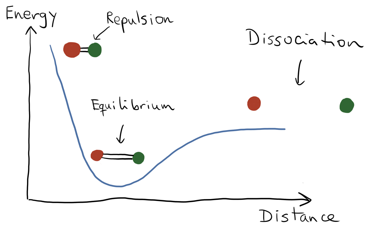
Illustration of a potential energy surface for a diatomic molecule.
Bond dissociation in a Hydrogen molecule
We now construct a potential energy surface and use it to compute equilibrium bond lengths and the bond dissociation energy. We begin with the simplest of molecules: \(H_2\). The formation or breaking of the \(H-H\) bond is also the most elementary of all reactions:
Using a minimal basis set, this molecular system can be described by two electrons in four spin-orbitals. When mapped to a qubit representation, we need a total of four qubits. The Hartree-Fock (HF) state is represented as \(|1100\rangle\), where the two lowest-energy orbitals are occupied, and the remaining two are unoccupied.
We design a quantum circuit consisting of SingleExcitation and
DoubleExcitation gates applied to the Hartree-Fock state. This circuit
will be optimized to prepare ground states for different configurations of the molecule.
import pennylane as qml
from pennylane import qchem

# Hartree-Fock state
hf = qml.qchem.hf_state(electrons=2, orbitals=4)
To construct the potential energy surface, we vary the location of the nuclei and calculate the energy for each resulting geometry of the molecule. We keep an \(H\) atom fixed at the origin and change only the coordinate of the other atom in a single direction. The potential energy surface is then a one-dimensional function depending only on the bond length, i.e., the separation between the atoms. For each value of the bond length, we construct the corresponding Hamiltonian, then optimize the circuit using gradient descent to obtain the ground-state energy. We vary the bond length in the range \(0.5\) to \(5.0\) Bohrs in steps of \(0.25\) Bohr. This covers the point where the \(H-H\) bond is formed, the equilibrium bond length, and the point where the bond is broken, which occurs when the atoms are far away from each other.
from pennylane import numpy as np

# atomic symbols defining the molecule
symbols = ['H', 'H']

# list to store energies
energies = []

# set up a loop to change bond length
r_range = np.arange(0.5, 5.0, 0.25)

# keeps track of points in the potential energy surface
pes_point = 0
We build the Hamiltonian using the molecular_hamiltonian()
function, and use standard Pennylane techniques to optimize the circuit.
for r in r_range:
    # Change only the z coordinate of one atom
    coordinates = np.array([0.0, 0.0, 0.0, 0.0, 0.0, r])

    # Obtain the qubit Hamiltonian
    H, qubits = qchem.molecular_hamiltonian(symbols, coordinates, method='pyscf')

    # define the device, optimizer and circuit
    dev = qml.device("default.qubit", wires=qubits)
    opt = qml.GradientDescentOptimizer(stepsize=0.4)

    @qml.qnode(dev, interface='autograd')
    def circuit(parameters):
        # Prepare the HF state: |1100>
        qml.BasisState(hf, wires=range(qubits))
        qml.DoubleExcitation(parameters[0], wires=[0, 1, 2, 3])
        qml.SingleExcitation(parameters[1], wires=[0, 2])
        qml.SingleExcitation(parameters[2], wires=[1, 3])

        return qml.expval(H)  # we are interested in minimizing this expectation value

    # initialize the gate parameters
    params = np.zeros(3, requires_grad=True)

    # initialize with converged parameters from previous point
    if pes_point > 0:
        params = params_old

    prev_energy = 0.0
    for n in range(50):
        # perform optimization step
        params, energy = opt.step_and_cost(circuit, params)

        if np.abs(energy - prev_energy) < 1e-6:
            break
        prev_energy = energy

    # store the converged parameters
    params_old = params
    pes_point = pes_point + 1

    energies.append(energy)
Let’s plot the results 📈
import matplotlib.pyplot as plt

fig, ax = plt.subplots()
ax.plot(r_range, energies)

ax.set(
    xlabel="Bond length (Bohr)",
    ylabel="Total energy (Hartree)",
    title="Potential energy surface for H$_2$ dissociation",
)
ax.grid()
plt.show()
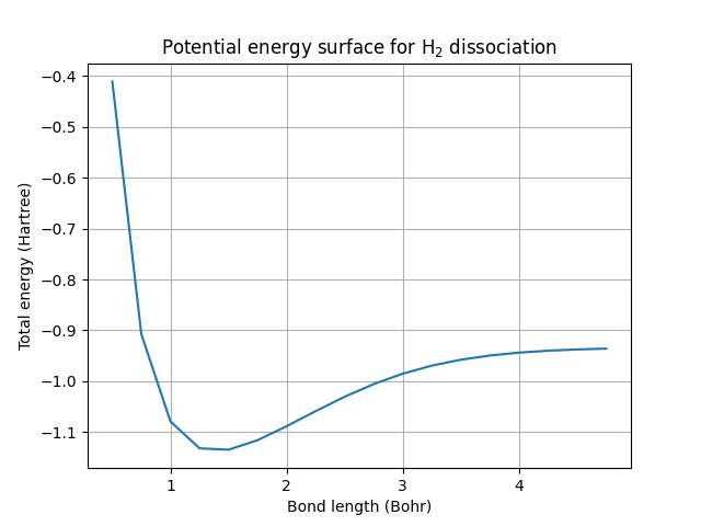
This is the potential energy surface for the dissociation of a hydrogen molecule into two hydrogen atoms. It is a numerical calculation of the same type of plot that was illustrated in the beginning. In a diatomic molecule such as \(H_2\), it can be used to obtain the equilibrium bond length — the distance between the two atoms that minimizes the total electronic energy. This is simply the minimum of the curve. We can also obtain the bond dissociation energy, which is the difference in the energy of the system when the atoms are far apart and the energy at equilibrium. At sufficiently large separations, the atoms no longer form a molecule, and the system is called “dissociated”.
Let’s use our results to compute the equilibrium bond length and the bond dissociation energy:
# equilibrium energy
e_eq = min(energies)
# energy when atoms are far apart
e_dis = energies[-1]

# Bond dissociation energy
bond_energy = e_dis - e_eq

# Equilibrium bond length
idx = energies.index(e_eq)
bond_length = r_range[idx]

print(f"The equilibrium bond length is {bond_length:.1f} Bohrs")
print(f"The bond dissociation energy is {bond_energy:.6f} Hartrees")
Out:
The equilibrium bond length is 1.5 Bohrs
The bond dissociation energy is 0.198772 Hartrees
These estimates can be improved by using bigger basis sets and extrapolating to the complete basis set limit 1. The calculations are of course are subject to the grid size of interatomic distances considered. The finer the grid size, the better the estimates.
Note
Did you notice a trick we used to speed up the calculations? The converged gate parameters for a particular geometry on the PES are used as the initial guess for the calculation at the adjacent geometry. With a better guess, the algorithm converges faster and we save considerable time.
Hydrogen Exchange Reaction
After studying a simple diatomic bond dissociation, we move to a slightly more complicated case: a hydrogen exchange reaction.
This reaction has a barrier, the transition state, that must be crossed for the exchange of an atom to be complete. In this case, the transition state corresponds to a specific linear arrangement of the atoms where one \(H-H\) bond is partially broken and the other \(H-H\) bond is partially formed. The molecular movie ⚛️🎥 below is an illustration of the reaction trajectory. It depicts how the distance between the hydrogen atoms changes as one bond is broken and another one is formed. The path along which the reaction proceeds is known as the reaction coordinate.
In a minimal basis like STO-3G, this system consists of three electrons in six spin molecular orbitals. This translates into a six-qubit problem, for which the Hartree-Fock state is \(|111000\rangle\). As there is an unpaired electron, the spin multiplicity is equal to two and needs to be specified, since it differs from the default value of one.
symbols = ["H", "H", "H"]
multiplicity = 2
To build a potential energy surface for the hydrogen exchange, we fix the positions of the
outermost atoms, and change only the placement of the middle atom. For this circuit, we employ all
single and double excitation gates, which can be conveniently done with the
AllSinglesDoubles template. The rest of the procedure follows as before.
from pennylane.templates import AllSinglesDoubles

energies = []
pes_point = 0

# get all the singles and doubles excitations, and Hartree-Fock state
electrons = 3
orbitals = 6
singles, doubles = qchem.excitations(electrons, orbitals)
hf = qml.qchem.hf_state(electrons, orbitals)


# loop to change reaction coordinate
r_range = np.arange(1.0, 3.0, 0.1)
for r in r_range:

    coordinates = np.array([0.0, 0.0, 0.0, 0.0, 0.0, r, 0.0, 0.0, 4.0])

    # We now specify the multiplicity
    H, qubits = qchem.molecular_hamiltonian(symbols, coordinates, mult=multiplicity, method='pyscf')

    dev = qml.device("default.qubit", wires=qubits)
    opt = qml.GradientDescentOptimizer(stepsize=1.5)

    @qml.qnode(dev, interface='autograd')
    def circuit(parameters):
        AllSinglesDoubles(parameters, range(qubits), hf, singles, doubles)
        return qml.expval(H)  # we are interested in minimizing this expectation value

    params = np.zeros(len(singles) + len(doubles), requires_grad=True)

    if pes_point > 0:
        params = params_old

    prev_energy = 0.0

    for n in range(60):
        params, energy = opt.step_and_cost(circuit, params)
        if np.abs(energy - prev_energy) < 1e-6:
            break
        prev_energy = energy

    # store the converged parameters
    params_old = params
    pes_point = pes_point + 1

    energies.append(energy)
Once the calculation is complete, we can plot the resulting potential energy surface.
fig, ax = plt.subplots()
ax.plot(r_range, energies)

ax.set(
    xlabel="Distance (Bohr)",
    ylabel="Total energy (Hartree)",
)
ax.grid()
plt.show()
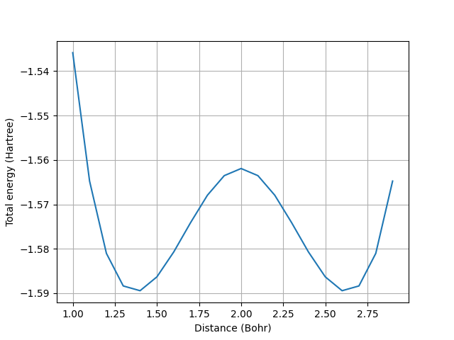
The two minima in the curve represent the energy of the reactants and products. The transition state is represented by the local maximum. These are the configurations illustrated in the animation above.
Activation energy barriers and reaction rates
The potential energy surfaces we computed so far can be leveraged for other important tasks, such as computing activation energy barriers and reaction rates. The activation energy barrier ( \(E_{a}\)) is defined as the difference between the energy of the reactants and the energy of the transition state.
This can be computed from the potential energy surface:
# Energy of the reactants and products - two minima on the PES
e_eq1 = min(energies)
e_eq2 = min([x for x in energies if x != e_eq1])

idx1 = energies.index(e_eq1)
idx2 = energies.index(e_eq2)

# Transition state is the local maximum between reactant and products
idx_min = min(idx1, idx2)
idx_max = max(idx1, idx2)

# Transition state energy
energy_ts = max(energies[idx_min:idx_max])

# Activation energy
activation_energy = energy_ts - e_eq1

print(f"The activation energy is {activation_energy:.6f} Hartrees")
Out:
The activation energy is 0.027504 Hartrees
The reaction rate constant (\(k\)) has an exponential dependence on the activation energy barrier, as shown in the Arrhenius equation (Arrr! 🏴☠️):
where \(k_B\) is the Boltzmann constant, \(T\) is the temperature, and \(A\) is a pre-exponential factor that can be determined empirically for each reaction. Crucially, the rate at which a chemical reaction occurs depends exponentially on the activation energy computed from the PES — this is a good reminder of the importance of performing highly-accurate calculations in quantum chemistry!
For example, let’s calculate the ratio of reaction rates when the temperature is doubled. We have
We choose \(T=300\) Kelvin, which is essentially room temperature. This makes doubling the temperature roughly equivalent to the temperature inside a pizza oven. We have
# convert to joules
activation_energy *= 4.36e-18
# Boltzmann constant in Joules/Kelvin
k_B = 1.38e-23
# Temperature
T = 300

ratio = np.exp(activation_energy / (2 * k_B * T))

print(f"Ratio of reaction rates is {ratio:.0f}")
Out:
Ratio of reaction rates is 1948918
Doubling the temperature can increase the rate by a factor of almost two million! For a similar reason, changing the activation energy can lead to drastic changes in the reaction rates, which means we have to be careful to compute it very accurately.
Conclusion
We can learn how atoms combine to form different molecules by performing experiments; this is the approach many of us learn as children by playing with chemistry sets. However, a deeper quantitative understanding of chemical reactions can be achieved by performing theoretical simulations of the mechanisms for forming and breaking bonds. This tutorial described how simple chemical reactions can be simulated using quantum algorithms that reconstruct potential energy surfaces, allowing us to identify reactants and products as minima of the energy, and transition states as local maxima. These results can then be used to calculate activation energies and reaction rates. The goal (and challenge!) for quantum computing is to improve both hardware and algorithms to reach the regime where providing accurate simulations becomes intractable for existing methods. If successful, this quest will allow us to understand the properties of quantum systems in ways that have so far been out of reach.
References
- 1
Mario Motta, Tanvi Gujarati, and Julia Rice, “A Tale of Colliding Electrons: Boosting the Accuracy of Chemical Simulations on Quantum Computers” (2020).
About the authors

Varun Rishi

Juan Miguel Arrazola
Total running time of the script: ( 1 minutes 7.766 seconds)