Note
Click here to download the full example code
Adaptive circuits for quantum chemistry
Author: Soran Jahangiri — Posted: 13 September 2021. Last updated: 10 April 2023
The key component of variational quantum algorithms for quantum chemistry is the circuit used to prepare electronic ground states of a molecule. The variational quantum eigensolver (VQE) 1, 2 is the method of choice for performing such quantum chemistry simulations on quantum devices with few qubits. For a given molecule, the appropriate circuit can be generated by using a pre-selected wavefunction ansatz, for example, the unitary coupled cluster with single and double excitations (UCCSD) 3. In this approach, we include all possible single and double excitations of electrons from the occupied spin-orbitals of a reference state to the unoccupied spin-orbitals 4. This makes the construction of the ansatz straightforward for any given molecule. However, using a pre-constructed ansatz has the disadvantage of reducing performance in favour of generality: the approach may work well in many cases, but it will not be optimized for a specific problem.
In practical applications, including all possible excitations usually increases the cost of the simulations without improving the accuracy of the results. This motivates implementing a strategy that allows for approximation of the contribution of the excitations and selects only those excitations that are found to be important for the given molecule. This can be done by using adaptive methods to construct a circuit for each given problem 5. Using adaptive circuits helps improve performance at the cost of reducing generality.
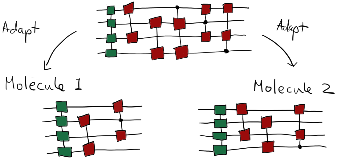
Examples of selecting specific gates to generate adaptive circuits.
In this tutorial, you will learn how to adaptively build customized quantum chemistry circuits to perform ADAPT-VQE 5 simulations. This includes a recipe to adaptively select gates that have a significant contribution to the desired state, while neglecting those that have a small contribution. You will also learn how to use PennyLane to leverage the sparsity of a molecular Hamiltonian to make the computation of the expectation values even more efficient. Let’s get started!
Adaptive circuits
The main idea behind building adaptive circuits is to compute the gradients with respect to all possible excitation gates and then select gates based on the magnitude of the computed gradients.
There are different ways to make use of the gradient information and here we discuss one of these strategies and apply it to compute the ground state energy of LiH. This method requires constructing the Hamiltonian and determining all possible excitations, which we can do with functionality built into PennyLane. But we first need to define the molecular parameters, including atomic symbols and coordinates. Note that the atomic coordinates are in Bohr.
import pennylane as qml
from pennylane import qchem
from pennylane import numpy as np
import time

symbols = ["Li", "H"]
geometry = np.array([0.0, 0.0, 0.0, 0.0, 0.0, 2.969280527])
We now compute the molecular Hamiltonian in the STO-3G basis and obtain the electronic excitations. We restrict ourselves to single and double excitations, but higher-level ones such as triple and quadruple excitations can be considered as well. Each of these electronic excitations is represented by a gate that excites electrons from the occupied orbitals of a reference state to the unoccupied ones. This allows us to prepare a state that is a superposition of the reference state and all of the excited states.
H, qubits = qchem.molecular_hamiltonian(
    symbols,
    geometry,
    active_electrons=2,
    active_orbitals=5
)

active_electrons = 2

singles, doubles = qchem.excitations(active_electrons, qubits)

print(f"Total number of excitations = {len(singles) + len(doubles)}")
Out:
Total number of excitations = 24
Note that we have a total of 24 excitations which can be represented by the same number of
excitation gates 4. Let’s now use an AdaptiveOptimizer
implemented in PennyLane to construct an adaptive circuit.
Adaptive Optimizer
The adaptive optimizer
grows an input quantum circuit by adding and optimizing gates selected from a user-defined
collection of operators. The algorithm first appends all of the gates provided in the initial
operator pool and computes the circuit gradients with respect to the gate parameters. It retains
the gate which has the largest gradient and then optimizes its parameter.
The process of growing the circuit can be repeated until the computed gradients converge to zero.
Let’s use AdaptiveOptimizer to perform an ADAPT-VQE 5
simulation and build an adaptive circuit for LiH.
We first create the operator pool which contains all single and double excitations.
singles_excitations = [qml.SingleExcitation(0.0, x) for x in singles]
doubles_excitations = [qml.DoubleExcitation(0.0, x) for x in doubles]
operator_pool = doubles_excitations + singles_excitations
We now define an initial circuit that prepares a Hartree-Fock state and returns the expectation value of the Hamiltonian. We also need to define a device.
hf_state = qchem.hf_state(active_electrons, qubits)
dev = qml.device("default.qubit", wires=qubits)
@qml.qnode(dev)
def circuit():
    [qml.PauliX(i) for i in np.nonzero(hf_state)[0]]
    return qml.expval(H)
We instantiate the optimizer and use it to build the circuit adaptively.
opt = qml.optimize.AdaptiveOptimizer()
for i in range(len(operator_pool)):
    circuit, energy, gradient = opt.step_and_cost(circuit, operator_pool)
    if i % 3 == 0:
        print("n = {:},  E = {:.8f} H, Largest Gradient = {:.3f}".format(i, energy, gradient))
        print(qml.draw(circuit, decimals=None)())
        print()
    if gradient < 3e-3:
        break
Out:
n = 0,  E = -7.86266588 H, Largest Gradient = 0.124
0: ──X─╭G²─┤ ╭<𝓗>
1: ──X─├G²─┤ ├<𝓗>
2: ────│───┤ ├<𝓗>
3: ────│───┤ ├<𝓗>
4: ────│───┤ ├<𝓗>
5: ────│───┤ ├<𝓗>
6: ────│───┤ ├<𝓗>
7: ────│───┤ ├<𝓗>
8: ────├G²─┤ ├<𝓗>
9: ────╰G²─┤ ╰<𝓗>

n = 3,  E = -7.88038372 H, Largest Gradient = 0.020
0: ──X─╭G²─╭G²─╭G²─╭G²─┤ ╭<𝓗>
1: ──X─├G²─├G²─├G²─├G²─┤ ├<𝓗>
2: ────│───├G²─│───│───┤ ├<𝓗>
3: ────│───│───├G²─│───┤ ├<𝓗>
4: ────│───│───│───│───┤ ├<𝓗>
5: ────│───│───│───│───┤ ├<𝓗>
6: ────│───│───│───├G²─┤ ├<𝓗>
7: ────│───│───│───╰G²─┤ ├<𝓗>
8: ────├G²─│───╰G²─────┤ ├<𝓗>
9: ────╰G²─╰G²─────────┤ ╰<𝓗>

n = 6,  E = -7.88189085 H, Largest Gradient = 0.006
0: ──X─╭G²─╭G²─╭G²─╭G²─╭G²─╭G²─╭G²─┤ ╭<𝓗>
1: ──X─├G²─├G²─├G²─├G²─├G²─├G²─├G²─┤ ├<𝓗>
2: ────│───├G²─│───│───│───├G²─│───┤ ├<𝓗>
3: ────│───│───├G²─│───│───╰G²─├G²─┤ ├<𝓗>
4: ────│───│───│───│───├G²─────│───┤ ├<𝓗>
5: ────│───│───│───│───╰G²─────│───┤ ├<𝓗>
6: ────│───│───│───├G²─────────│───┤ ├<𝓗>
7: ────│───│───│───╰G²─────────│───┤ ├<𝓗>
8: ────├G²─│───╰G²─────────────╰G²─┤ ├<𝓗>
9: ────╰G²─╰G²─────────────────────┤ ╰<𝓗>

n = 9,  E = -7.88199765 H, Largest Gradient = 0.005
0: ──X─╭G²─╭G²─╭G²─╭G²─╭G²─╭G²─╭G²─╭G²─╭G²─╭G─┤ ╭<𝓗>
1: ──X─├G²─├G²─├G²─├G²─├G²─├G²─├G²─├G²─├G²─│──┤ ├<𝓗>
2: ────│───├G²─│───│───│───├G²─│───│───├G²─╰G─┤ ├<𝓗>
3: ────│───│───├G²─│───│───╰G²─├G²─│───│──────┤ ├<𝓗>
4: ────│───│───│───│───├G²─────│───│───│──────┤ ├<𝓗>
5: ────│───│───│───│───╰G²─────│───│───│──────┤ ├<𝓗>
6: ────│───│───│───├G²─────────│───│───│──────┤ ├<𝓗>
7: ────│───│───│───╰G²─────────│───│───│──────┤ ├<𝓗>
8: ────├G²─│───╰G²─────────────╰G²─├G²─│──────┤ ├<𝓗>
9: ────╰G²─╰G²─────────────────────╰G²─╰G²────┤ ╰<𝓗>

n = 12,  E = -7.88217789 H, Largest Gradient = 0.003
0: ──X─╭G²─╭G²─╭G²─╭G²─╭G²─╭G²─╭G²─╭G²─╭G²─╭G────╭G²─╭G─┤ ╭<𝓗>
1: ──X─├G²─├G²─├G²─├G²─├G²─├G²─├G²─├G²─├G²─│──╭G─├G²─│──┤ ├<𝓗>
2: ────│───├G²─│───│───│───├G²─│───│───├G²─╰G─│──├G²─╰G─┤ ├<𝓗>
3: ────│───│───├G²─│───│───╰G²─├G²─│───│──────╰G─╰G²────┤ ├<𝓗>
4: ────│───│───│───│───├G²─────│───│───│────────────────┤ ├<𝓗>
5: ────│───│───│───│───╰G²─────│───│───│────────────────┤ ├<𝓗>
6: ────│───│───│───├G²─────────│───│───│────────────────┤ ├<𝓗>
7: ────│───│───│───╰G²─────────│───│───│────────────────┤ ├<𝓗>
8: ────├G²─│───╰G²─────────────╰G²─├G²─│────────────────┤ ├<𝓗>
9: ────╰G²─╰G²─────────────────────╰G²─╰G²──────────────┤ ╰<𝓗>

n = 15,  E = -7.88226581 H, Largest Gradient = 0.003
0: ──X─╭G²─╭G²─╭G²─╭G²─╭G²─╭G²─╭G²─╭G²─╭G²─╭G────╭G²─╭G─╭G²────╭G²─┤ ╭<𝓗>
1: ──X─├G²─├G²─├G²─├G²─├G²─├G²─├G²─├G²─├G²─│──╭G─├G²─│──├G²─╭G─├G²─┤ ├<𝓗>
2: ────│───├G²─│───│───│───├G²─│───│───├G²─╰G─│──├G²─╰G─├G²─│──│───┤ ├<𝓗>
3: ────│───│───├G²─│───│───╰G²─├G²─│───│──────╰G─╰G²────│───╰G─├G²─┤ ├<𝓗>
4: ────│───│───│───│───├G²─────│───│───│────────────────│──────│───┤ ├<𝓗>
5: ────│───│───│───│───╰G²─────│───│───│────────────────│──────│───┤ ├<𝓗>
6: ────│───│───│───├G²─────────│───│───│────────────────│──────│───┤ ├<𝓗>
7: ────│───│───│───╰G²─────────│───│───│────────────────│──────│───┤ ├<𝓗>
8: ────├G²─│───╰G²─────────────╰G²─├G²─│────────────────│──────╰G²─┤ ├<𝓗>
9: ────╰G²─╰G²─────────────────────╰G²─╰G²──────────────╰G²────────┤ ╰<𝓗>
The resulting energy matches the exact energy of the ground electronic state of LiH, which is
-7.8825378193 Ha, within chemical accuracy. Note that some of the gates appear more than once in
the circuit. By default, AdaptiveOptimizer does not eliminate the selected
gates from the pool. We can set drain_pool=True to prevent repetition of the gates by
removing the selected gate from the operator pool.
@qml.qnode(dev)
def circuit():
    [qml.PauliX(i) for i in np.nonzero(hf_state)[0]]
    return qml.expval(H)

opt = qml.optimize.AdaptiveOptimizer()
for i in range(len(operator_pool)):
    circuit, energy, gradient = opt.step_and_cost(circuit, operator_pool, drain_pool=True)
    if i % 2 == 0:
        print("n = {:},  E = {:.8f} H, Largest Gradient = {:.3f}".format(i, energy, gradient))
        print(qml.draw(circuit, decimals=None)())
        print()
    if gradient < 3e-3:
        break
Out:
n = 0,  E = -7.86266588 H, Largest Gradient = 0.124
0: ──X─╭G²─┤ ╭<𝓗>
1: ──X─├G²─┤ ├<𝓗>
2: ────│───┤ ├<𝓗>
3: ────│───┤ ├<𝓗>
4: ────│───┤ ├<𝓗>
5: ────│───┤ ├<𝓗>
6: ────│───┤ ├<𝓗>
7: ────│───┤ ├<𝓗>
8: ────├G²─┤ ├<𝓗>
9: ────╰G²─┤ ╰<𝓗>

n = 2,  E = -7.87869588 H, Largest Gradient = 0.035
0: ──X─╭G²─╭G²─╭G²─┤ ╭<𝓗>
1: ──X─├G²─├G²─├G²─┤ ├<𝓗>
2: ────│───├G²─│───┤ ├<𝓗>
3: ────│───│───├G²─┤ ├<𝓗>
4: ────│───│───│───┤ ├<𝓗>
5: ────│───│───│───┤ ├<𝓗>
6: ────│───│───│───┤ ├<𝓗>
7: ────│───│───│───┤ ├<𝓗>
8: ────├G²─│───╰G²─┤ ├<𝓗>
9: ────╰G²─╰G²─────┤ ╰<𝓗>

n = 4,  E = -7.88095806 H, Largest Gradient = 0.019
0: ──X─╭G²─╭G²─╭G²─╭G²─╭G²─┤ ╭<𝓗>
1: ──X─├G²─├G²─├G²─├G²─├G²─┤ ├<𝓗>
2: ────│───├G²─│───│───│───┤ ├<𝓗>
3: ────│───│───├G²─│───│───┤ ├<𝓗>
4: ────│───│───│───│───├G²─┤ ├<𝓗>
5: ────│───│───│───│───╰G²─┤ ├<𝓗>
6: ────│───│───│───├G²─────┤ ├<𝓗>
7: ────│───│───│───╰G²─────┤ ├<𝓗>
8: ────├G²─│───╰G²─────────┤ ├<𝓗>
9: ────╰G²─╰G²─────────────┤ ╰<𝓗>

n = 6,  E = -7.88189085 H, Largest Gradient = 0.004
0: ──X─╭G²─╭G²─╭G²─╭G²─╭G²─╭G²─╭G─┤ ╭<𝓗>
1: ──X─├G²─├G²─├G²─├G²─├G²─├G²─│──┤ ├<𝓗>
2: ────│───├G²─│───│───│───├G²─╰G─┤ ├<𝓗>
3: ────│───│───├G²─│───│───╰G²────┤ ├<𝓗>
4: ────│───│───│───│───├G²────────┤ ├<𝓗>
5: ────│───│───│───│───╰G²────────┤ ├<𝓗>
6: ────│───│───│───├G²────────────┤ ├<𝓗>
7: ────│───│───│───╰G²────────────┤ ├<𝓗>
8: ────├G²─│───╰G²────────────────┤ ├<𝓗>
9: ────╰G²─╰G²────────────────────┤ ╰<𝓗>

n = 8,  E = -7.88200088 H, Largest Gradient = 0.001
0: ──X─╭G²─╭G²─╭G²─╭G²─╭G²─╭G²─╭G────╭G─┤ ╭<𝓗>
1: ──X─├G²─├G²─├G²─├G²─├G²─├G²─│──╭G─│──┤ ├<𝓗>
2: ────│───├G²─│───│───│───├G²─╰G─│──│──┤ ├<𝓗>
3: ────│───│───├G²─│───│───╰G²────╰G─│──┤ ├<𝓗>
4: ────│───│───│───│───├G²───────────│──┤ ├<𝓗>
5: ────│───│───│───│───╰G²───────────│──┤ ├<𝓗>
6: ────│───│───│───├G²───────────────│──┤ ├<𝓗>
7: ────│───│───│───╰G²───────────────│──┤ ├<𝓗>
8: ────├G²─│───╰G²───────────────────╰G─┤ ├<𝓗>
9: ────╰G²─╰G²──────────────────────────┤ ╰<𝓗>
Manual construction
We can also build adaptive circuits manually by adding groups of gates one at a time. We follow these steps:
Compute gradients for all double excitations.
Select the double excitations with gradients larger than a pre-defined threshold.
Perform VQE to obtain the optimized parameters for the selected double excitations.
Repeat steps 1 and 2 for the single excitations.
Perform the final VQE optimization with all the selected excitations.
We create a circuit that applies a selected group of gates to the reference Hartree-Fock state.
def circuit_1(params, excitations):
    qml.BasisState(hf_state, wires=range(qubits))

    for i, excitation in enumerate(excitations):
        if len(excitation) == 4:
            qml.DoubleExcitation(params[i], wires=excitation)
        else:
            qml.SingleExcitation(params[i], wires=excitation)
    return qml.expval(H)
We now construct our first group of gates by including all the double excitations and compute the gradient for each one. We also need to define a cost function. We initialize the parameter values to zero such that the gradients are computed with respect to the Hartree-Fock state.
dev = qml.device("default.qubit", wires=qubits)
cost_fn = qml.QNode(circuit_1, dev, interface="autograd")

circuit_gradient = qml.grad(cost_fn, argnum=0)

params = [0.0] * len(doubles)
grads = circuit_gradient(params, excitations=doubles)

for i in range(len(doubles)):
    print(f"Excitation : {doubles[i]}, Gradient: {grads[i]}")
Out:
Excitation : [0, 1, 2, 3], Gradient: -0.012782168180745634
Excitation : [0, 1, 2, 5], Gradient: 0.0
Excitation : [0, 1, 2, 7], Gradient: 0.0
Excitation : [0, 1, 2, 9], Gradient: 0.034264503599058194
Excitation : [0, 1, 3, 4], Gradient: 0.0
Excitation : [0, 1, 3, 6], Gradient: 0.0
Excitation : [0, 1, 3, 8], Gradient: -0.03426450359905819
Excitation : [0, 1, 4, 5], Gradient: -0.023581524379110933
Excitation : [0, 1, 4, 7], Gradient: 0.0
Excitation : [0, 1, 4, 9], Gradient: 0.0
Excitation : [0, 1, 5, 6], Gradient: 0.0
Excitation : [0, 1, 5, 8], Gradient: 0.0
Excitation : [0, 1, 6, 7], Gradient: -0.02358152437912184
Excitation : [0, 1, 6, 9], Gradient: 0.0
Excitation : [0, 1, 7, 8], Gradient: 0.0
Excitation : [0, 1, 8, 9], Gradient: -0.12362273289626591
The computed gradients have different values, reflecting the contribution of each gate in the final state prepared by the circuit. Many of the gradient values are zero and we select those gates that have a gradient above a pre-defined threshold, which we set to \(10^{-5}\).
doubles_select = [doubles[i] for i in range(len(doubles)) if abs(grads[i]) > 1.0e-5]
doubles_select
Out:
[[0, 1, 2, 3], [0, 1, 2, 9], [0, 1, 3, 8], [0, 1, 4, 5], [0, 1, 6, 7], [0, 1, 8, 9]]
There are only 6 double excitation gates, out of the original 16, that have gradients above the threshold. We add the selected gates to the circuit and optimize it to determine the updated parameters for the selected gates. We also need to define an optimizer. Note that the optimization is not very costly as we only have six gates in our circuit.
opt = qml.GradientDescentOptimizer(stepsize=0.5)

params_doubles = np.zeros(len(doubles_select), requires_grad=True)

for n in range(20):
    params_doubles = opt.step(cost_fn, params_doubles, excitations=doubles_select)
Now, we keep the selected gates in the circuit and compute the gradients with respect to all of the single excitation gates, selecting those that have a non-negligible gradient. To do that, we need to slightly modify our circuit such that parameters of the double excitation gates are kept fixed while the gradients are computed for the single excitation gates.
def circuit_2(params, excitations, gates_select, params_select):
    qml.BasisState(hf_state, wires=range(qubits))

    for i, gate in enumerate(gates_select):
        if len(gate) == 4:
            qml.DoubleExcitation(params_select[i], wires=gate)
        elif len(gate) == 2:
            qml.SingleExcitation(params_select[i], wires=gate)

    for i, gate in enumerate(excitations):
        if len(gate) == 4:
            qml.DoubleExcitation(params[i], wires=gate)
        elif len(gate) == 2:
            qml.SingleExcitation(params[i], wires=gate)
    return qml.expval(H)
We now compute the gradients for the single excitation gates.
cost_fn = qml.QNode(circuit_2, dev, interface="autograd")
circuit_gradient = qml.grad(cost_fn, argnum=0)
params = [0.0] * len(singles)

grads = circuit_gradient(
    params,
    excitations=singles,
    gates_select=doubles_select,
    params_select=params_doubles
)

for i in range(len(singles)):
    print(f"Excitation : {singles[i]}, Gradient: {grads[i]}")
Out:
Excitation : [0, 2], Gradient: -0.005062544629162135
Excitation : [0, 4], Gradient: 0.0
Excitation : [0, 6], Gradient: 0.0
Excitation : [0, 8], Gradient: -0.0009448055879242643
Excitation : [1, 3], Gradient: 0.004926625112977095
Excitation : [1, 5], Gradient: 0.0
Excitation : [1, 7], Gradient: 0.0
Excitation : [1, 9], Gradient: 0.0014535553867884928
Similar to the double excitation gates, we select those single excitations that have a gradient larger than a predefined threshold.
singles_select = [singles[i] for i in range(len(singles)) if abs(grads[i]) > 1.0e-5]
singles_select
Out:
[[0, 2], [0, 8], [1, 3], [1, 9]]
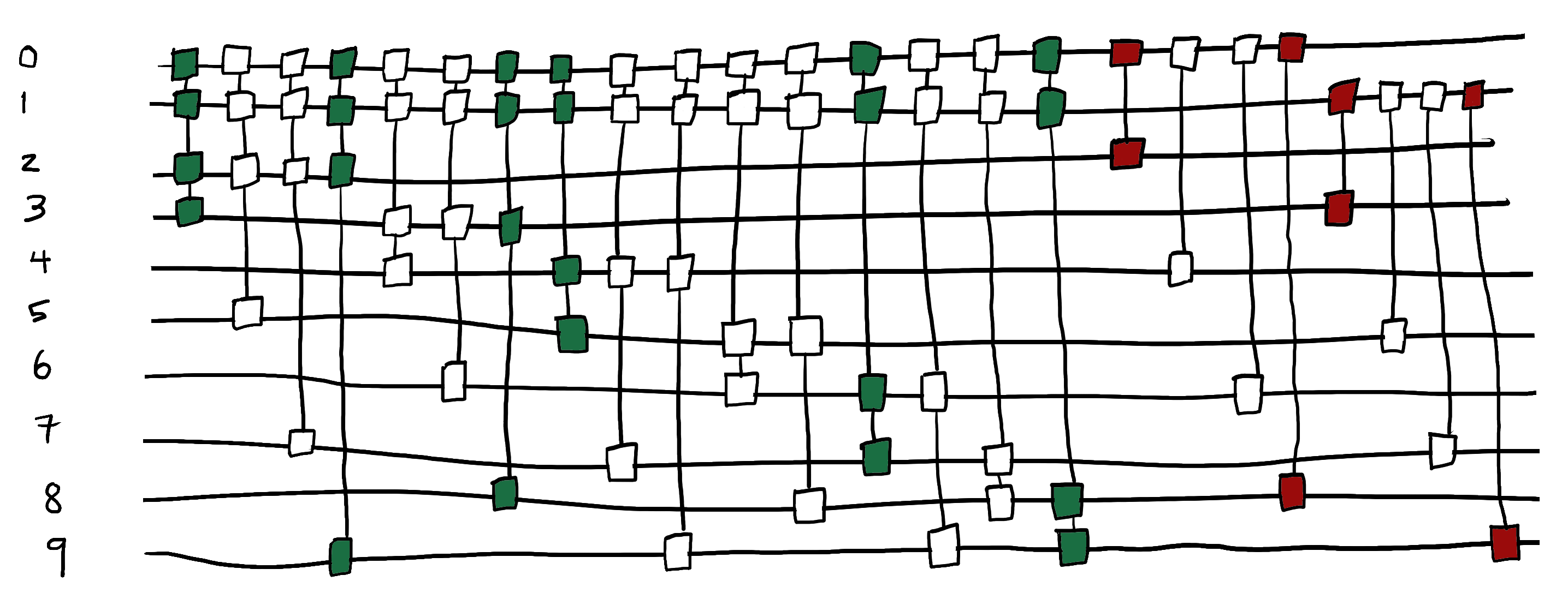
We now have all of the gates we need to build our circuit. The selected single and double excitation gates are highlighted in the figure below.
We perform a final circuit optimization to get the ground-state energy. The resulting energy should match the exact energy of the ground electronic state of LiH which is -7.8825378193 Ha.
cost_fn = qml.QNode(circuit_1, dev, interface="autograd")

params = np.zeros(len(doubles_select + singles_select), requires_grad=True)

gates_select = doubles_select + singles_select

for n in range(20):
    t1 = time.time()
    params, energy = opt.step_and_cost(cost_fn, params, excitations=gates_select)
    t2 = time.time()
    print("n = {:},  E = {:.8f} H, t = {:.2f} s".format(n, energy, t2 - t1))
Out:
n = 0,  E = -7.86266588 H, t = 0.72 s
n = 1,  E = -7.87094622 H, t = 0.72 s
n = 2,  E = -7.87563101 H, t = 0.86 s
n = 3,  E = -7.87829148 H, t = 0.72 s
n = 4,  E = -7.87981707 H, t = 0.72 s
n = 5,  E = -7.88070478 H, t = 0.72 s
n = 6,  E = -7.88123144 H, t = 0.85 s
n = 7,  E = -7.88155162 H, t = 0.72 s
n = 8,  E = -7.88175219 H, t = 0.72 s
n = 9,  E = -7.88188238 H, t = 0.86 s
n = 10,  E = -7.88197042 H, t = 0.72 s
n = 11,  E = -7.88203269 H, t = 0.72 s
n = 12,  E = -7.88207881 H, t = 0.72 s
n = 13,  E = -7.88211453 H, t = 0.85 s
n = 14,  E = -7.88214336 H, t = 0.72 s
n = 15,  E = -7.88216745 H, t = 0.72 s
n = 16,  E = -7.88218815 H, t = 0.85 s
n = 17,  E = -7.88220635 H, t = 0.72 s
n = 18,  E = -7.88222262 H, t = 0.72 s
n = 19,  E = -7.88223735 H, t = 0.72 s
Success! We obtained the ground state energy of LiH, within chemical accuracy, by having only 10 gates in our circuit. This is less than half of the total number of single and double excitations of LiH (24).
Sparse Hamiltonians
Molecular Hamiltonians and quantum states are sparse. For instance, let’s look at the Hamiltonian
we built for LiH. We can compute its matrix representation in the computational basis using the
Hamiltonian function sparse_matrix(). This function
returns the matrix in the SciPy sparse coordinate format.
H_sparse = H.sparse_matrix()
H_sparse
Out:
<1024x1024 sparse matrix of type '<class 'numpy.complex128'>'
    with 11776 stored elements in Compressed Sparse Row format>
The matrix has \(1024^2=1,048,576\) entries, but only \(11264\) of them are non-zero.
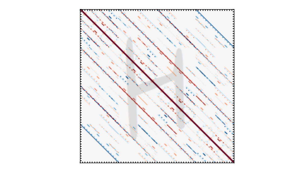
Matrix representation of the LiH Hamiltonian in the computational basis.
Leveraging this sparsity can significantly reduce the simulation times. We use the implemented functionality in PennyLane for computing the expectation value of the sparse Hamiltonian observable. This can reduce the cost of simulations by orders of magnitude depending on the size of the molecule. We use the selected gates obtained in the previous steps and perform the final optimization step with the sparse method. Note that the sparse method currently only works with the parameter-shift differentiation method.
excitations = doubles_select + singles_select

params = np.zeros(len(excitations), requires_grad=True)

@qml.qnode(dev, diff_method="parameter-shift", interface="autograd")
def circuit(params):
    qml.BasisState(hf_state, wires=range(qubits))

    for i, excitation in enumerate(excitations):
        if len(excitation) == 4:
            qml.DoubleExcitation(params[i], wires=excitation)
        elif len(excitation) == 2:
            qml.SingleExcitation(params[i], wires=excitation)

    return qml.expval(qml.SparseHamiltonian(H_sparse, wires=range(qubits)))


for n in range(20):
    t1 = time.time()
    params, energy = opt.step_and_cost(circuit, params)
    t2 = time.time()
    print("n = {:},  E = {:.8f} H, t = {:.2f} s".format(n, energy[0], t2 - t1))
Out:
n = 0,  E = -7.86266588 H, t = 0.13 s
n = 1,  E = -7.87094622 H, t = 0.13 s
n = 2,  E = -7.87563101 H, t = 0.13 s
n = 3,  E = -7.87829148 H, t = 0.13 s
n = 4,  E = -7.87981707 H, t = 0.13 s
n = 5,  E = -7.88070478 H, t = 0.26 s
n = 6,  E = -7.88123144 H, t = 0.13 s
n = 7,  E = -7.88155162 H, t = 0.13 s
n = 8,  E = -7.88175219 H, t = 0.13 s
n = 9,  E = -7.88188238 H, t = 0.13 s
n = 10,  E = -7.88197042 H, t = 0.13 s
n = 11,  E = -7.88203269 H, t = 0.13 s
n = 12,  E = -7.88207881 H, t = 0.13 s
n = 13,  E = -7.88211453 H, t = 0.13 s
n = 14,  E = -7.88214336 H, t = 0.13 s
n = 15,  E = -7.88216745 H, t = 0.13 s
n = 16,  E = -7.88218815 H, t = 0.13 s
n = 17,  E = -7.88220635 H, t = 0.13 s
n = 18,  E = -7.88222262 H, t = 0.13 s
n = 19,  E = -7.88223735 H, t = 0.13 s
Using the sparse method reproduces the ground state energy while the optimization time is much shorter. The average iteration time for the sparse method is about 18 times smaller than that of the original non-sparse approach. The performance of the sparse optimization will be even better for larger molecules.
Conclusions
We have learned that building quantum chemistry circuits adaptively and using the functionality for sparse objects makes molecular simulations significantly more efficient. We learned how to use an adaptive optimizer implemented in PennyLane, that selects the gates one at time, to perform ADAPT-VQE 5 simulations. We also followed an adaptive strategy that selects a group of gates based on information about the gradients.
References
- 1
A. Peruzzo, J. McClean et al., “A variational eigenvalue solver on a photonic quantum processor”. Nat. Commun. 5, 4213 (2014).
- 2
Y. Cao, J. Romero, et al., “Quantum Chemistry in the Age of Quantum Computing”. Chem. Rev. 2019, 119, 19, 10856-10915.
- 3
J. Romero, R. Babbush, et al., “Strategies for quantum computing molecular energies using the unitary coupled cluster ansatz”. arXiv:1701.02691
- 4(1,2)
- 5(1,2,3,4)
H. R. Grimsley, S. E. Economou, E. Barnes, N. J. Mayhall, “An adaptive variational algorithm for exact molecular simulations on a quantum computer”. Nat. Commun. 2019, 10, 3007.