Optimization of molecular geometries

Author: Alain Delgado — Posted: 30 June 2021. Last updated: 25 June 2022.

Predicting the most stable arrangement of atoms in a molecule is one of the most important tasks in quantum chemistry. Essentially, this is an optimization problem where the total energy of the molecule is minimized with respect to the positions of the atomic nuclei. The molecular geometry obtained from this calculation is in fact the starting point for many simulations of molecular properties. If the geometry is inaccurate, then any calculations that rely on it may also be inaccurate.

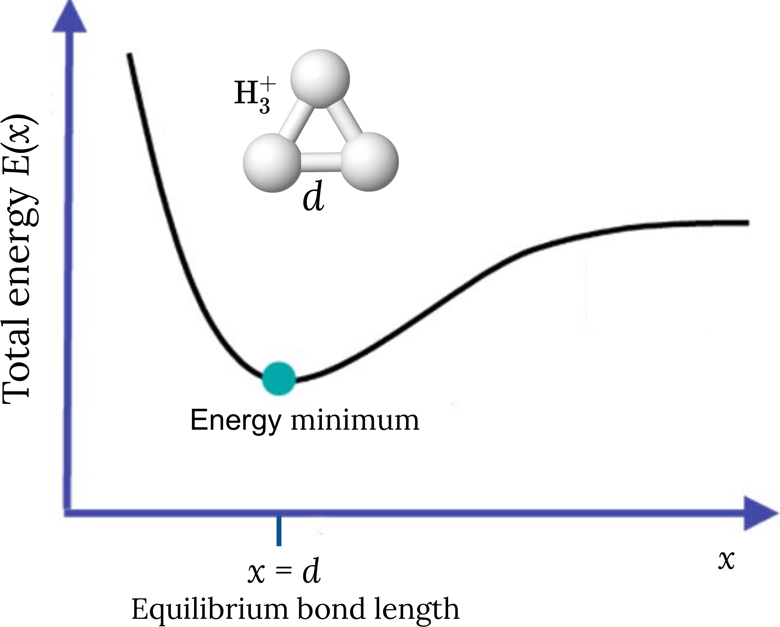
Since the nuclei are much heavier than the electrons, we can treat them as point particles clamped to their positions. Under this assumption, the total energy of the molecule \(E(x)\) depends on the nuclear coordinates \(x\), which define the potential energy surface. Solving the stationary problem \(\nabla_x E(x) = 0\) corresponds to molecular geometry optimization and the optimized nuclear coordinates determine the equilibrium geometry of the molecule. The figure below illustrates these concepts for the trihydrogen cation. Its equilibrium geometry in the electronic ground state corresponds to the minimum energy of the potential energy surface. At this minimum, the three hydrogen atoms are located at the vertices of an equilateral triangle whose side length is the optimized bond length \(d\).

In this tutorial, you will learn how to recast the problem of finding the equilibrium geometry of a molecule in terms of a general variational quantum algorithm. The central idea is to consider explicitly that the target electronic Hamiltonian \(H(x)\) is a parametrized observable that depends on the nuclear coordinates \(x\). This implies that the objective function, defined by the expectation value of the Hamiltonian computed in the trial state prepared by a quantum computer, depends on both the quantum circuit and the Hamiltonian parameters.

The quantum algorithm in a nutshell

The goal of the variational algorithm is to find the global minimum of the cost function \(g(\theta, x) = \langle \Psi(\theta) \vert H(x) \vert \Psi(\theta) \rangle\) with respect to the circuit parameters \(\theta\) and the nuclear coordinates \(x\) entering the electronic Hamiltonian of the molecule. To that end, we use a gradient-descent method and follow a joint optimization scheme where the gradients of the cost function with respect to circuit and Hamiltonian parameters are simultaneously computed at each step. This approach does not require nested optimization of the state parameters for each set of nuclear coordinates, as occurs in classical algorithms for molecular geometry optimization, where the energy minimum is searched for along the potential energy surface of the electronic state 1.

In this tutorial we demonstrate how to use PennyLane to implement quantum optimization of molecular geometries. The algorithm consists of the following steps:

1. Build the parametrized electronic Hamiltonian \(H(x)\) of the molecule.

2. Design the variational quantum circuit to prepare the electronic trial state of the molecule, \(\vert \Psi(\theta) \rangle\).

3. Define the cost function \(g(\theta, x) = \langle \Psi(\theta) \vert H(x) \vert \Psi(\theta) \rangle\).

4. Initialize the variational parameters \(\theta\) and \(x\). Perform a joint optimization of the circuit and Hamiltonian parameters to minimize the cost function \(g(\theta, x)\). The gradient with respect to the circuit parameters can be obtained using a variety of established methods, which are natively supported in PennyLane. The gradients with respect to the nuclear coordinates can be computed using the formula

   \[\nabla_x g(\theta, x) = \langle \Psi(\theta) \vert \nabla_x H(x) \vert \Psi(\theta) \rangle.\]

Once the optimization is finalized, the circuit parameters determine the energy of the electronic state, and the nuclear coordinates determine the equilibrium geometry of the molecule in this state.

Let’s get started! ⚛️

Building the parametrized electronic Hamiltonian

In this example, we want to optimize the geometry of the trihydrogen cation \(\mathrm{H}_3^+\), described in a minimal basis set, where two electrons are shared between three hydrogen atoms (see figure above). The molecule is specified by providing a list with the symbols of the atomic species and a one-dimensional array with the initial set of nuclear coordinates in atomic units .

from pennylane import numpy as np

symbols = ["H", "H", "H"]
x = np.array([0.028, 0.054, 0.0, 0.986, 1.610, 0.0, 1.855, 0.002, 0.0], requires_grad=True)

Next, we need to build the parametrized electronic Hamiltonian \(H(x)\). We use the Jordan-Wigner transformation 2 to represent the fermionic Hamiltonian as a linear combination of Pauli operators,

\[H(x) = \sum_j h_j(x) \prod_i^{N} \sigma_i^{(j)}.\]

The expansion coefficients \(h_j(x)\) carry the dependence on the coordinates \(x\), the operators \(\sigma_i\) represent the Pauli group \(\{I, X, Y, Z\}\), and \(N\) is the number of qubits required to represent the electronic wave function.

We define the function H(x) to build the parametrized Hamiltonian of the trihydrogen cation using the molecular_hamiltonian() function.

import pennylane as qml


def H(x):
    return qml.qchem.molecular_hamiltonian(symbols, x, charge=1)[0]

The variational quantum circuit

Here, we describe the second step of the quantum algorithm: define the quantum circuit to prepare the electronic ground-state \(\vert \Psi(\theta)\rangle\) of the \(\mathrm{H}_3^+\) molecule.

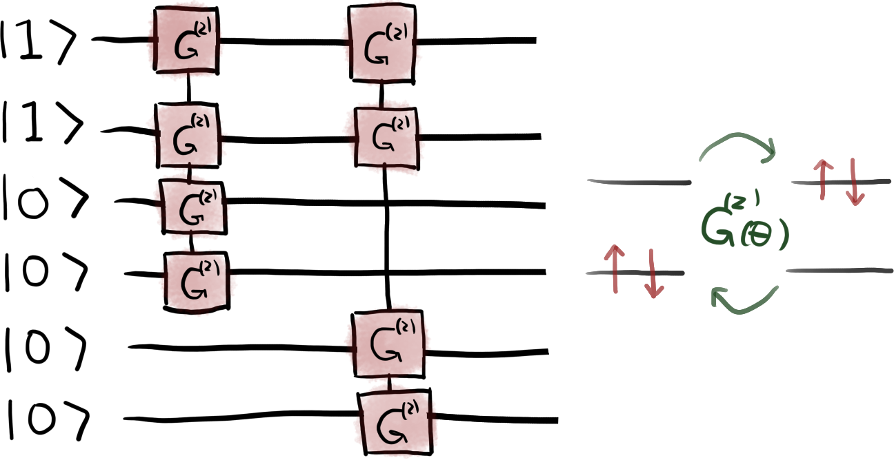
Six qubits are required to encode the occupation number of the molecular spin-orbitals. To capture the effects of electronic correlations 3, we need to prepare the \(N\)-qubit system in a superposition of the Hartree-Fock state \(\vert 110000 \rangle\) with other states that differ by a double- or single-excitation. For example, the state \(\vert 000011 \rangle\) is obtained by exciting two particles from qubits 0, 1 to 4, 5. Similarly, the state \(\vert 011000 \rangle\) corresponds to a single excitation from qubit 0 to 2. This can be done using the single-excitation and double-excitation gates \(G\) and \(G^{(2)}\) 4 implemented in the form of Givens rotations in PennyLane. For more details see the tutorial Givens rotations for quantum chemistry.

In addition, we use an adaptive algorithm 6 to select the excitation operations included in the variational quantum circuit. The algorithm proceeds as follows:

1. Generate the indices of the qubits involved in all single- and double-excitations. For example, the indices of the singly-excited state \(\vert 011000 \rangle\) are given by the list [0, 2]. Similarly, the indices of the doubly-excited state \(\vert 000011 \rangle\) are [0, 1, 4, 5].

2. Construct the circuit using all double-excitation gates. Compute the gradient of the cost function \(g(\theta, x)\) with respect to each double-excitation gate and retain only those with non-zero gradient.

3. Include the selected double-excitation gates and repeat the process for the single-excitation gates.

4. Build the final variational quantum circuit by including the selected gates.

For the \(\mathrm{H}_3^+\) molecule in a minimal basis set we have a total of eight excitations of the reference state. After applying the adaptive algorithm the final quantum circuit contains only two double-excitation operations that act on the qubits [0, 1, 2, 3] and [0, 1, 4, 5]. The circuit is illustrated in the figure below.

To implement this quantum circuit, we use the hf_state() function to generate the occupation-number vector representing the Hartree-Fock state

hf = qml.qchem.hf_state(electrons=2, orbitals=6)
print(hf)

Out:

[1 1 0 0 0 0]

The hf array is used by the BasisState operation to initialize the qubit register. Then, the DoubleExcitation operations are applied First, we define the quantum device used to compute the expectation value. In this example, we use the default.qubit simulator:

num_wires = 6
dev = qml.device("default.qubit", wires=num_wires)


@qml.qnode(dev, interface="autograd")
def circuit(params, obs, wires):
    qml.BasisState(hf, wires=wires)
    qml.DoubleExcitation(params[0], wires=[0, 1, 2, 3])
    qml.DoubleExcitation(params[1], wires=[0, 1, 4, 5])

    return qml.expval(obs)

This circuit prepares the trial state

\[\vert\Psi(\theta_1, \theta_2)\rangle = \mathrm{cos}(\theta_1)\mathrm{cos}(\theta_2)\vert110000\rangle - \mathrm{cos}(\theta_1)\mathrm{sin}(\theta_2)\vert000011\rangle - \mathrm{sin}(\theta_1)\vert001100\rangle,\]

where \(\theta_1\) and \(\theta_2\) are the circuit parameters that need to be optimized to find the ground-state energy of the molecule.

The cost function and the nuclear gradients

The third step of the algorithm is to define the cost function \(g(\theta, x) = \langle \Psi(\theta) \vert H(x) \vert\Psi(\theta) \rangle\). It evaluates the expectation value of the parametrized Hamiltonian \(H(x)\) in the trial state \(\vert\Psi(\theta)\rangle\).

Next, we define the cost function \(g(\theta, x)\) which depends on both the circuit and the Hamiltonian parameters. Specifically we consider the expectation values of the Hamiltonian.

def cost(params, x):
    hamiltonian = H(x)
    return circuit(params, obs=hamiltonian, wires=range(num_wires))

We minimize the cost function \(g(\theta, x)\) using a gradient-based method, and compute the gradients with respect to both the circuit parameters \(\theta\) and the nuclear coordinates \(x\). The circuit gradients are computed analytically using the automatic differentiation techniques available in PennyLane. The nuclear gradients are evaluated by taking the expectation value of the gradient of the electronic Hamiltonian,

\[\nabla_x g(\theta, x) = \langle \Psi(\theta) \vert \nabla_x H(x) \vert \Psi(\theta) \rangle.\]

We use the finite_diff() function to compute the gradient of the Hamiltonian using a central-difference approximation. Then, we evaluate the expectation value of the gradient components \(\frac{\partial H(x)}{\partial x_i}\). This is implemented by the function grad_x:

def finite_diff(f, x, delta=0.01):
    """Compute the central-difference finite difference of a function"""
    gradient = []

    for i in range(len(x)):
        shift = np.zeros_like(x)
        shift[i] += 0.5 * delta
        res = (f(x + shift) - f(x - shift)) * delta**-1
        gradient.append(res)

    return gradient


def grad_x(params, x):
    grad_h = finite_diff(H, x)
    grad = [circuit(params, obs=obs, wires=range(num_wires)) for obs in grad_h]
    return np.array(grad)

Optimization of the molecular geometry

Finally, we proceed to minimize our cost function to find the ground state equilibrium geometry of the \(\mathrm{H}_3^+\) molecule. As a reminder, the circuit parameters and the nuclear coordinates will be jointly optimized at each optimization step. This approach does not require nested VQE optimization of the circuit parameters for each set of nuclear coordinates.

We start by defining the classical optimizers:

opt_theta = qml.GradientDescentOptimizer(stepsize=0.4)
opt_x = qml.GradientDescentOptimizer(stepsize=0.8)

Next, we initialize the circuit parameters \(\theta\). The angles \(\theta_1\) and \(\theta_2\) are set to zero so that the initial state \(\vert\Psi(\theta_1, \theta_2)\rangle\) is the Hartree-Fock state.

theta = np.array([0.0, 0.0], requires_grad=True)

The initial set of nuclear coordinates \(x\), defined at the beginning of the tutorial, was computed classically within the Hartree-Fock approximation using the GAMESS program 5. This is a natural choice for the starting geometry that we are aiming to improve due to the electronic correlation effects included in the trial state \(\vert\Psi(\theta)\rangle\).

We carry out the optimization over a maximum of 100 steps. The circuit parameters and the nuclear coordinates are optimized until the maximum component of the nuclear gradient \(\nabla_x g(\theta,x)\) is less than or equal to \(10^{-5}\) Hartree/Bohr. Typically, this is the convergence criterion used for optimizing molecular geometries in quantum chemistry simulations.

from functools import partial

# store the values of the cost function
energy = []

# store the values of the bond length
bond_length = []

# Factor to convert from Bohrs to Angstroms
bohr_angs = 0.529177210903

for n in range(100):

    # Optimize the circuit parameters
    theta.requires_grad = True
    x.requires_grad = False
    theta, _ = opt_theta.step(cost, theta, x)

    # Optimize the nuclear coordinates
    x.requires_grad = True
    theta.requires_grad = False
    _, x = opt_x.step(cost, theta, x, grad_fn=grad_x)

    energy.append(cost(theta, x))
    bond_length.append(np.linalg.norm(x[0:3] - x[3:6]) * bohr_angs)

    if n % 4 == 0:
        print(f"Step = {n},  E = {energy[-1]:.8f} Ha,  bond length = {bond_length[-1]:.5f} A")

    # Check maximum component of the nuclear gradient
    if np.max(grad_x(theta, x)) <= 1e-05:
        break

print("\n" f"Final value of the ground-state energy = {energy[-1]:.8f} Ha")
print("\n" "Ground-state equilibrium geometry")
print("%s %4s %8s %8s" % ("symbol", "x", "y", "z"))
for i, atom in enumerate(symbols):
    print(f"  {atom}    {x[3 * i]:.4f}   {x[3 * i + 1]:.4f}   {x[3 * i + 2]:.4f}")

Out:

Step = 0,  E = -1.26094338 Ha,  bond length = 0.96762 A
Step = 4,  E = -1.27360653 Ha,  bond length = 0.97619 A
Step = 8,  E = -1.27437809 Ha,  bond length = 0.98223 A
Step = 12,  E = -1.27443305 Ha,  bond length = 0.98457 A
Step = 16,  E = -1.27443729 Ha,  bond length = 0.98533 A
Step = 20,  E = -1.27443763 Ha,  bond length = 0.98556 A
Step = 24,  E = -1.27443766 Ha,  bond length = 0.98563 A

Final value of the ground-state energy = -1.27443766 Ha

Ground-state equilibrium geometry
symbol    x        y        z
  H    0.0102   0.0442   0.0000
  H    0.9867   1.6303   0.0000
  H    1.8720   -0.0085   0.0000

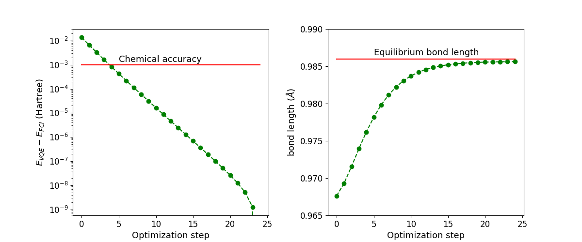
Next, we plot the values of the ground state energy of the molecule and the bond length as a function of the optimization step.

import matplotlib.pyplot as plt

fig = plt.figure()
fig.set_figheight(5)
fig.set_figwidth(12)

# Add energy plot on column 1
E_fci = -1.27443765658
E_vqe = np.array(energy)
ax1 = fig.add_subplot(121)
ax1.plot(range(n + 1), E_vqe - E_fci, "go-", ls="dashed")
ax1.plot(range(n + 1), np.full(n + 1, 0.001), color="red")
ax1.set_xlabel("Optimization step", fontsize=13)
ax1.set_ylabel("$E_{VQE} - E_{FCI}$ (Hartree)", fontsize=13)
ax1.text(5, 0.0013, r"Chemical accuracy", fontsize=13)
plt.yscale("log")
plt.xticks(fontsize=12)
plt.yticks(fontsize=12)

# Add bond length plot on column 2
d_fci = 0.986
ax2 = fig.add_subplot(122)
ax2.plot(range(n + 1), bond_length, "go-", ls="dashed")
ax2.plot(range(n + 1), np.full(n + 1, d_fci), color="red")
ax2.set_ylim([0.965, 0.99])
ax2.set_xlabel("Optimization step", fontsize=13)
ax2.set_ylabel("bond length ($\AA$)", fontsize=13)
ax2.text(5, 0.9865, r"Equilibrium bond length", fontsize=13)
plt.xticks(fontsize=12)
plt.yticks(fontsize=12)

plt.subplots_adjust(wspace=0.3)
plt.show()

Out:

/home/runner/work/qml/qml/demonstrations/tutorial_mol_geo_opt.py:367: UserWarning: linestyle is redundantly defined by the 'linestyle' keyword argument and the fmt string "go-" (-> linestyle='-'). The keyword argument will take precedence.
  ax1.plot(range(n + 1), E_vqe - E_fci, "go-", ls="dashed")
/home/runner/work/qml/qml/demonstrations/tutorial_mol_geo_opt.py:379: UserWarning: linestyle is redundantly defined by the 'linestyle' keyword argument and the fmt string "go-" (-> linestyle='-'). The keyword argument will take precedence.
  ax2.plot(range(n + 1), bond_length, "go-", ls="dashed")

Notice that despite the fact that the ground-state energy is already converged within chemical accuracy (\(0.0016\) Ha) after the fourth iteration, more optimization steps are required to find the equilibrium bond length of the molecule.

The figure below animates snapshots of the atomic structure of the trihydrogen cation as the quantum algorithm was searching for the equilibrium geometry. For visualization purposes, the initial nuclear coordinates were generated by perturbing the HF geometry. The quantum algorithm is able to find the correct equilibrium geometry of the \(\mathrm{H}_3^+\) molecule where the three H atoms are located at the vertices of an equilateral triangle.

To summarize, we have shown how the scope of variational quantum algorithms can be extended to perform quantum simulations of molecules involving both the electronic and the nuclear degrees of freedom. The joint optimization scheme described here is a generalization of the usual VQE algorithm where only the electronic state is parametrized. Extending the applicability of the variational quantum algorithms to target parametrized Hamiltonians could be also relevant to simulate the optical properties of molecules where the fermionic observables depend also on the electric field of the incoming radiation 7.

References

1

F. Jensen. “Introduction to computational chemistry”. (John Wiley & Sons, 2016).

2

Jacob T. Seeley, Martin J. Richard, Peter J. Love. “The Bravyi-Kitaev transformation for quantum computation of electronic structure”. Journal of Chemical Physics 137, 224109 (2012).

3

Jorge Kohanoff. “Electronic structure calculations for solids and molecules: theory and computational methods”. (Cambridge University Press, 2006).

4

J.M. Arrazola, O. Di Matteo, N. Quesada, S. Jahangiri, A. Delgado, N. Killoran. “Universal quantum circuits for quantum chemistry”. arXiv:2106.13839, (2021)

5

M.W. Schmidt, K.K. Baldridge, J.A. Boatz, S.T. Elbert, M.S. Gordon, J.H. Jensen, S. Koseki, N. Matsunaga, K.A. Nguyen, S.Su, et al. “General atomic and molecular electronic structure system”. Journal of Computational Chemistry 14, 1347 (1993)

6

A. Delgado, J.M. Arrazola, S. Jahangiri, Z. Niu, J. Izaac, C. Roberts, N. Killoran. “Variational quantum algorithm for molecular geometry optimization”. arXiv:2106.13840, (2021)

7

P. Pulay. “Analytical derivative methods in quantum chemistry”. Advances in Chemical Sciences (1987)

About the author

Alain Delgado

Alain Delgado Gran is a senior quantum scientist working at Xanadu. He has a background in quantum many-body systems and electronic structure methods. His work focuses on the application of quantum algorithms for simulating advanced materials.

demos/tutorial_mol_geo_opt

 

Download Python script

 

Download Notebook

 

View on GitHub