Data-reuploading classifier

Author: Shahnawaz Ahmed — Posted: 11 October 2019. Last updated: 19 January 2021.

A single-qubit quantum circuit which can implement arbitrary unitary operations can be used as a universal classifier much like a single hidden-layered Neural Network. As surprising as it sounds, Pérez-Salinas et al. (2019) discuss this with their idea of ‘data reuploading’. It is possible to load a single qubit with arbitrary dimensional data and then use it as a universal classifier.

In this example, we will implement this idea with Pennylane - a python based tool for quantum machine learning, automatic differentiation, and optimization of hybrid quantum-classical computations.

Background

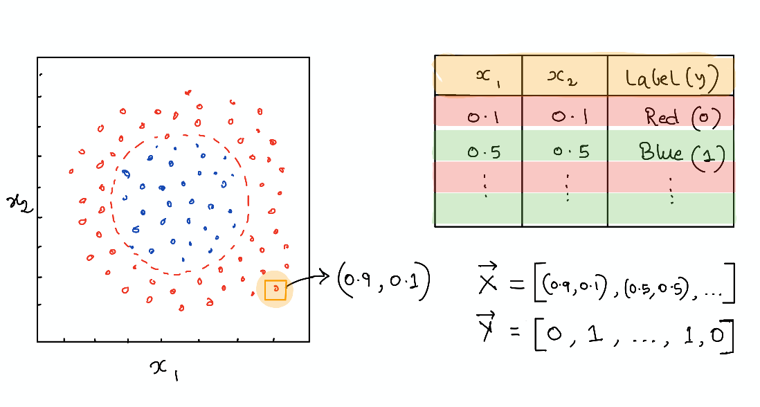
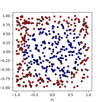
We consider a simple classification problem and will train a single-qubit variational quantum circuit to achieve this goal. The data is generated as a set of random points in a plane \((x_1, x_2)\) and labeled as 1 (blue) or 0 (red) depending on whether they lie inside or outside a circle. The goal is to train a quantum circuit to predict the label (red or blue) given an input point’s coordinate.

Transforming quantum states using unitary operations

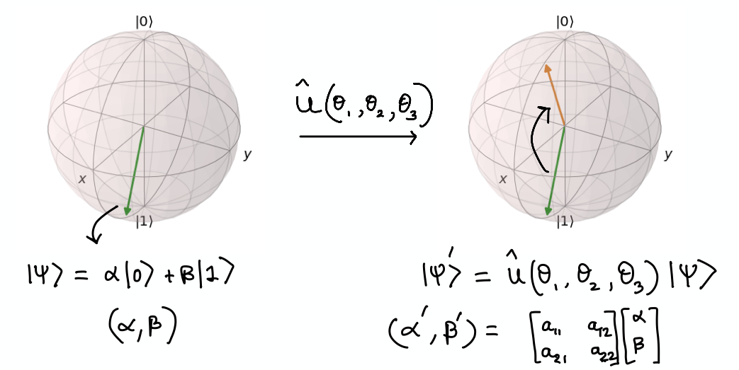
A single-qubit quantum state is characterized by a two-dimensional state vector and can be visualized as a point in the so-called Bloch sphere. Instead of just being a 0 (up) or 1 (down), it can exist in a superposition with say 30% chance of being in the \(|0 \rangle\) and 70% chance of being in the \(|1 \rangle\) state. This is represented by a state vector \(|\psi \rangle = \sqrt{0.3}|0 \rangle + \sqrt{0.7}|1 \rangle\) - the probability “amplitude” of the quantum state. In general we can take a vector \((\alpha, \beta)\) to represent the probabilities of a qubit being in a particular state and visualize it on the Bloch sphere as an arrow.

Data loading using unitaries

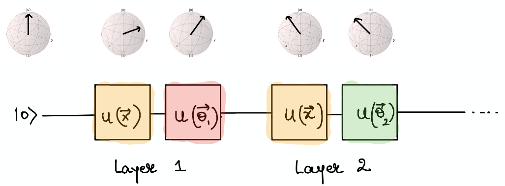
In order to load data onto a single qubit, we use a unitary operation \(U(x_1, x_2, x_3)\) which is just a parameterized matrix multiplication representing the rotation of the state vector in the Bloch sphere. E.g., to load \((x_1, x_2)\) into the qubit, we just start from some initial state vector, \(|0 \rangle\), apply the unitary operation \(U(x_1, x_2, 0)\) and end up at a new point on the Bloch sphere. Here we have padded 0 since our data is only 2D. Pérez-Salinas et al. (2019) discuss how to load a higher dimensional data point (\([x_1, x_2, x_3, x_4, x_5, x_6]\)) by breaking it down in sets of three parameters (\(U(x_1, x_2, x_3), U(x_4, x_5, x_6)\)).

Model parameters with data re-uploading

Once we load the data onto the quantum circuit, we want to have some trainable nonlinear model similar to a neural network as well as a way of learning the weights of the model from data. This is again done with unitaries, \(U(\theta_1, \theta_2, \theta_3)\), such that we load the data first and then apply the weights to form a single layer \(L(\vec \theta, \vec x) = U(\vec \theta)U(\vec x)\). In principle, this is just application of two matrix multiplications on an input vector initialized to some value. In order to increase the number of trainable parameters (similar to increasing neurons in a single layer of a neural network), we can reapply this layer again and again with new sets of weights, \(L(\vec \theta_1, \vec x) L(\vec \theta_2, , \vec x) ... L(\vec \theta_L, \vec x)\) for \(L\) layers. The quantum circuit would look like the following:

The cost function and “nonlinear collapse”

So far, we have only performed linear operations (matrix multiplications) and we know that we need to have some nonlinear squashing similar to activation functions in neural networks to really make a universal classifier (Cybenko 1989). Here is where things gets a bit quantum. After the application of the layers, we will end up at some point on the Bloch sphere due to the sequence of unitaries implementing rotations of the input. These are still just linear transformations of the input state. Now, the output of the model should be a class label which can be encoded as fixed vectors (Blue = \([1, 0]\), Red = \([0, 1]\)) on the Bloch sphere. We want to end up at either of them after transforming our input state through alternate applications of data layer and weights.

We can use the idea of the “collapse” of our quantum state into one or other class. This happens when we measure the quantum state which leads to its projection as either the state 0 or 1. We can compute the fidelity (or closeness) of the output state to the class label making the output state jump to either \(| 0 \rangle\) or \(|1\rangle\). By repeating this process several times, we can compute the probability or overlap of our output to both labels and assign a class based on the label our output has a higher overlap. This is much like having a set of output neurons and selecting the one which has the highest value as the label.

We can encode the output label as a particular quantum state that we want to end up in and use Pennylane to find the probability of ending up in that state after running the circuit. We construct an observable corresponding to the output label using the Hermitian operator. The expectation value of the observable gives the overlap or fidelity. We can then define the cost function as the sum of the fidelities for all the data points after passing through the circuit and optimize the parameters \((\vec \theta)\) to minimize the cost.

\[\texttt{Cost} = \sum_{\texttt{data points}} (1 - \texttt{fidelity}(\psi_{\texttt{output}}(\vec x, \vec \theta), \psi_{\texttt{label}}))\]

Now, we can use our favorite optimizer to maximize the sum of the fidelities over all data points (or batches of datapoints) and find the optimal weights for classification. Gradient-based optimizers such as Adam (Kingma et. al., 2014) can be used if we have a good model of the circuit and how noise might affect it. Or, we can use some gradient-free method such as L-BFGS (Liu, Dong C., and Nocedal, J., 1989) to evaluate the gradient and find the optimal weights where we can treat the quantum circuit as a black-box and the gradients are computed numerically using a fixed number of function evaluations and iterations. The L-BFGS method can be used with the PyTorch interface for Pennylane.

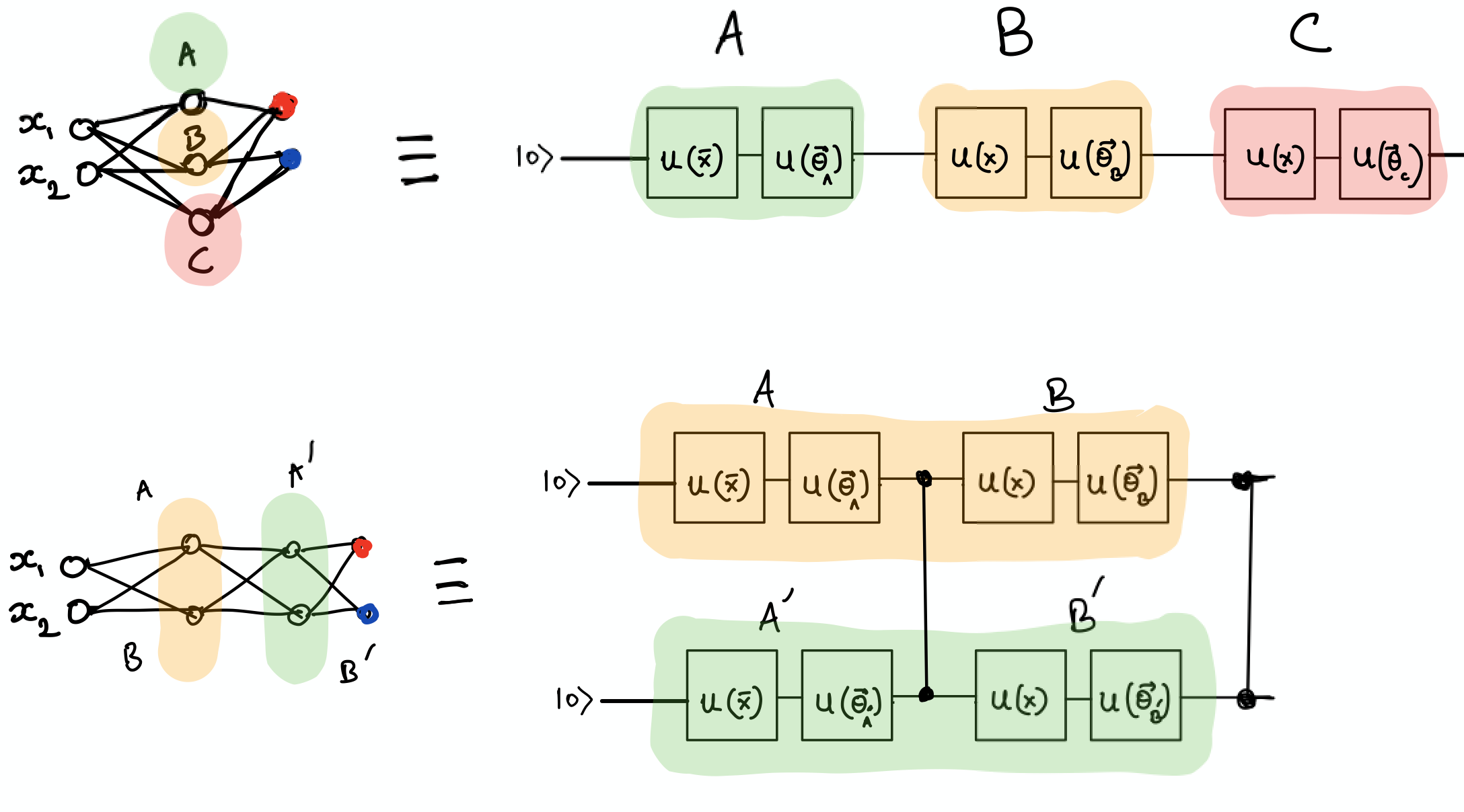
Multiple qubits, entanglement and Deep Neural Networks

The Universal Approximation Theorem declares that a neural network with two or more hidden layers can serve as a universal function approximator. Recently, we have witnessed remarkable progress of learning algorithms using Deep Neural Networks.

Pérez-Salinas et al. (2019) make a connection to Deep Neural Networks by describing that in their approach the “layers” \(L_i(\vec \theta_i, \vec x )\) are analogous to the size of the intermediate hidden layer of a neural network. And the concept of deep (multiple layers of the neural network) relates to the number of qubits. So, multiple qubits with entanglement between them could provide some quantum advantage over classical neural networks. But here, we will only implement a single qubit classifier.

“Talk is cheap. Show me the code.” - Linus Torvalds

import pennylane as qml
from pennylane import numpy as np
from pennylane.optimize import AdamOptimizer, GradientDescentOptimizer

import matplotlib.pyplot as plt


# Set a random seed
np.random.seed(42)


# Make a dataset of points inside and outside of a circle
def circle(samples, center=[0.0, 0.0], radius=np.sqrt(2 / np.pi)):
    """
    Generates a dataset of points with 1/0 labels inside a given radius.

    Args:
        samples (int): number of samples to generate
        center (tuple): center of the circle
        radius (float: radius of the circle

    Returns:
        Xvals (array[tuple]): coordinates of points
        yvals (array[int]): classification labels
    """
    Xvals, yvals = [], []

    for i in range(samples):
        x = 2 * (np.random.rand(2)) - 1
        y = 0
        if np.linalg.norm(x - center) < radius:
            y = 1
        Xvals.append(x)
        yvals.append(y)
    return np.array(Xvals, requires_grad=False), np.array(yvals, requires_grad=False)


def plot_data(x, y, fig=None, ax=None):
    """
    Plot data with red/blue values for a binary classification.

    Args:
        x (array[tuple]): array of data points as tuples
        y (array[int]): array of data points as tuples
    """
    if fig == None:
        fig, ax = plt.subplots(1, 1, figsize=(5, 5))
    reds = y == 0
    blues = y == 1
    ax.scatter(x[reds, 0], x[reds, 1], c="red", s=20, edgecolor="k")
    ax.scatter(x[blues, 0], x[blues, 1], c="blue", s=20, edgecolor="k")
    ax.set_xlabel("$x_1$")
    ax.set_ylabel("$x_2$")


Xdata, ydata = circle(500)
fig, ax = plt.subplots(1, 1, figsize=(4, 4))
plot_data(Xdata, ydata, fig=fig, ax=ax)
plt.show()


# Define output labels as quantum state vectors
def density_matrix(state):
    """Calculates the density matrix representation of a state.

    Args:
        state (array[complex]): array representing a quantum state vector

    Returns:
        dm: (array[complex]): array representing the density matrix
    """
    return state * np.conj(state).T


label_0 = [[1], [0]]
label_1 = [[0], [1]]
state_labels = np.array([label_0, label_1], requires_grad=False)

Simple classifier with data reloading and fidelity loss

dev = qml.device("default.qubit", wires=1)
# Install any pennylane-plugin to run on some particular backend


@qml.qnode(dev, interface="autograd")
def qcircuit(params, x, y):
    """A variational quantum circuit representing the Universal classifier.

    Args:
        params (array[float]): array of parameters
        x (array[float]): single input vector
        y (array[float]): single output state density matrix

    Returns:
        float: fidelity between output state and input
    """
    for p in params:
        qml.Rot(*x, wires=0)
        qml.Rot(*p, wires=0)
    return qml.expval(qml.Hermitian(y, wires=[0]))


def cost(params, x, y, state_labels=None):
    """Cost function to be minimized.

    Args:
        params (array[float]): array of parameters
        x (array[float]): 2-d array of input vectors
        y (array[float]): 1-d array of targets
        state_labels (array[float]): array of state representations for labels

    Returns:
        float: loss value to be minimized
    """
    # Compute prediction for each input in data batch
    loss = 0.0
    dm_labels = [density_matrix(s) for s in state_labels]
    for i in range(len(x)):
        f = qcircuit(params, x[i], dm_labels[y[i]])
        loss = loss + (1 - f) ** 2
    return loss / len(x)

Utility functions for testing and creating batches

def test(params, x, y, state_labels=None):
    """
    Tests on a given set of data.

    Args:
        params (array[float]): array of parameters
        x (array[float]): 2-d array of input vectors
        y (array[float]): 1-d array of targets
        state_labels (array[float]): 1-d array of state representations for labels

    Returns:
        predicted (array([int]): predicted labels for test data
        output_states (array[float]): output quantum states from the circuit
    """
    fidelity_values = []
    dm_labels = [density_matrix(s) for s in state_labels]
    predicted = []

    for i in range(len(x)):
        fidel_function = lambda y: qcircuit(params, x[i], y)
        fidelities = [fidel_function(dm) for dm in dm_labels]
        best_fidel = np.argmax(fidelities)

        predicted.append(best_fidel)
        fidelity_values.append(fidelities)

    return np.array(predicted), np.array(fidelity_values)


def accuracy_score(y_true, y_pred):
    """Accuracy score.

    Args:
        y_true (array[float]): 1-d array of targets
        y_predicted (array[float]): 1-d array of predictions
        state_labels (array[float]): 1-d array of state representations for labels

    Returns:
        score (float): the fraction of correctly classified samples
    """
    score = y_true == y_pred
    return score.sum() / len(y_true)


def iterate_minibatches(inputs, targets, batch_size):
    """
    A generator for batches of the input data

    Args:
        inputs (array[float]): input data
        targets (array[float]): targets

    Returns:
        inputs (array[float]): one batch of input data of length `batch_size`
        targets (array[float]): one batch of targets of length `batch_size`
    """
    for start_idx in range(0, inputs.shape[0] - batch_size + 1, batch_size):
        idxs = slice(start_idx, start_idx + batch_size)
        yield inputs[idxs], targets[idxs]

Train a quantum classifier on the circle dataset

# Generate training and test data
num_training = 200
num_test = 2000

Xdata, y_train = circle(num_training)
X_train = np.hstack((Xdata, np.zeros((Xdata.shape[0], 1), requires_grad=False)))

Xtest, y_test = circle(num_test)
X_test = np.hstack((Xtest, np.zeros((Xtest.shape[0], 1), requires_grad=False)))


# Train using Adam optimizer and evaluate the classifier
num_layers = 3
learning_rate = 0.6
epochs = 10
batch_size = 32

opt = AdamOptimizer(learning_rate, beta1=0.9, beta2=0.999)

# initialize random weights
params = np.random.uniform(size=(num_layers, 3), requires_grad=True)

predicted_train, fidel_train = test(params, X_train, y_train, state_labels)
accuracy_train = accuracy_score(y_train, predicted_train)

predicted_test, fidel_test = test(params, X_test, y_test, state_labels)
accuracy_test = accuracy_score(y_test, predicted_test)

# save predictions with random weights for comparison
initial_predictions = predicted_test

loss = cost(params, X_test, y_test, state_labels)

print(
    "Epoch: {:2d} | Cost: {:3f} | Train accuracy: {:3f} | Test Accuracy: {:3f}".format(
        0, loss, accuracy_train, accuracy_test
    )
)

for it in range(epochs):
    for Xbatch, ybatch in iterate_minibatches(X_train, y_train, batch_size=batch_size):
        params, _, _, _ = opt.step(cost, params, Xbatch, ybatch, state_labels)

    predicted_train, fidel_train = test(params, X_train, y_train, state_labels)
    accuracy_train = accuracy_score(y_train, predicted_train)
    loss = cost(params, X_train, y_train, state_labels)

    predicted_test, fidel_test = test(params, X_test, y_test, state_labels)
    accuracy_test = accuracy_score(y_test, predicted_test)
    res = [it + 1, loss, accuracy_train, accuracy_test]
    print(
        "Epoch: {:2d} | Loss: {:3f} | Train accuracy: {:3f} | Test accuracy: {:3f}".format(
            *res
        )
    )

Out:

Epoch:  0 | Cost: 0.415535 | Train accuracy: 0.460000 | Test Accuracy: 0.448500
Epoch:  1 | Loss: 0.125417 | Train accuracy: 0.840000 | Test accuracy: 0.804000
Epoch:  2 | Loss: 0.154322 | Train accuracy: 0.775000 | Test accuracy: 0.756000
Epoch:  3 | Loss: 0.145234 | Train accuracy: 0.810000 | Test accuracy: 0.799000
Epoch:  4 | Loss: 0.126142 | Train accuracy: 0.805000 | Test accuracy: 0.781500
Epoch:  5 | Loss: 0.127102 | Train accuracy: 0.845000 | Test accuracy: 0.794500
Epoch:  6 | Loss: 0.128556 | Train accuracy: 0.825000 | Test accuracy: 0.807000
Epoch:  7 | Loss: 0.113327 | Train accuracy: 0.810000 | Test accuracy: 0.794500
Epoch:  8 | Loss: 0.109549 | Train accuracy: 0.895000 | Test accuracy: 0.857000
Epoch:  9 | Loss: 0.147936 | Train accuracy: 0.750000 | Test accuracy: 0.750000
Epoch: 10 | Loss: 0.104038 | Train accuracy: 0.890000 | Test accuracy: 0.847000

Results

print(
    "Cost: {:3f} | Train accuracy {:3f} | Test Accuracy : {:3f}".format(
        loss, accuracy_train, accuracy_test
    )
)

print("Learned weights")
for i in range(num_layers):
    print("Layer {}: {}".format(i, params[i]))


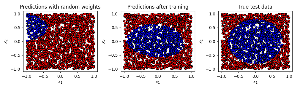
fig, axes = plt.subplots(1, 3, figsize=(10, 3))
plot_data(X_test, initial_predictions, fig, axes[0])
plot_data(X_test, predicted_test, fig, axes[1])
plot_data(X_test, y_test, fig, axes[2])
axes[0].set_title("Predictions with random weights")
axes[1].set_title("Predictions after training")
axes[2].set_title("True test data")
plt.tight_layout()
plt.show()

Out:

Cost: 0.104038 | Train accuracy 0.890000 | Test Accuracy : 0.847000
Learned weights
Layer 0: [-0.23838965  1.17081693 -0.19781887]
Layer 1: [0.64850867 0.71778245 0.46408056]
Layer 2: [ 2.39560597 -1.21404538  0.32099705]

References

[1] Pérez-Salinas, Adrián, et al. “Data re-uploading for a universal quantum classifier.” arXiv preprint arXiv:1907.02085 (2019).

[2] Kingma, Diederik P., and Ba, J. “Adam: A method for stochastic optimization.” arXiv preprint arXiv:1412.6980 (2014).

[3] Liu, Dong C., and Nocedal, J. “On the limited memory BFGS method for large scale optimization.” Mathematical programming 45.1-3 (1989): 503-528.

About the author

Shahnawaz Ahmed

Shahnawaz works on developing useful machine learning techniques for scientific applications with a focus on quantum information and computing.

demos/tutorial_data_reuploading_classifier

 

Download Python script

 

Download Notebook

 

View on GitHub