Differentiable Hartree-Fock

Author: Soran Jahangiri — Posted: 09 May 2022. Last updated: 09 May 2022.

In this tutorial, you will learn how to use PennyLane’s differentiable Hartree-Fock solver 1. The quantum chemistry module in PennyLane, qml.qchem, provides built-in methods for constructing atomic and molecular orbitals, building Fock matrices and solving the self-consistent field equations to obtain optimized orbitals which can be used to construct fully-differentiable molecular Hamiltonians. PennyLane allows users to natively compute derivatives of all these objects with respect to the underlying parameters using the methods of automatic differentiation. We introduce a workflow to jointly optimize circuit parameters, nuclear coordinates and basis set parameters in a variational quantum eigensolver algorithm. You will also learn how to visualize the atomic and molecular orbitals which can be used to create an animation like this:

The bonding molecular orbital of hydrogen visualized during a full geometry, circuit and basis set optimization.

Let’s get started!

Differentiable Hamiltonians

Variational quantum algorithms aim to calculate the energy of a molecule by constructing a parameterized quantum circuit and finding a set of parameters that minimize the expectation value of the electronic molecular Hamiltonian. The optimization can be carried out by computing the gradients of the expectation value with respect to these parameters and iteratively updating them until convergence is achieved. In principle, the optimization process is not limited to the circuit parameters and can be extended to include the parameters of the Hamiltonian that can be optimized concurrently with the circuit parameters. The aim is now to obtain the set of parameters that minimize the following expectation value

\[\left \langle \Psi(\theta) | H(\beta) | \Psi(\theta) \right \rangle,\]

where \(\theta\) and \(\beta\) represent the circuit and Hamiltonian parameters, respectively.

Computing the gradient of a molecular Hamiltonian is challenging because the dependency of the Hamiltonian on the molecular parameters is typically not very straightforward. This makes symbolic differentiation methods, which obtain derivatives of an input function by direct mathematical manipulation, of limited scope. Furthermore, numerical differentiation methods based on finite differences are not always reliable due to their intrinsic instability, especially when the number of differentiable parameters is large. These limitations can be alleviated by using automatic differentiation methods which can be used to compute exact gradients of a function, implemented with computer code, using resources comparable to those required to evaluate the function itself.

Efficient optimization of the molecular Hamiltonian parameters in a variational quantum algorithm is essential for tackling problems such as geometry optimization and vibrational frequency calculations. These problems require computing the first- and second-order derivatives of the molecular energy with respect to nuclear coordinates which can be efficiently obtained if the variational workflow is automatically differentiable. Another important example is the simultaneous optimization of the parameters of the basis set used to construct the atomic orbitals which can in principle increase the accuracy of the computed energy without increasing the number of qubits in a quantum simulation. The joint optimization of the circuit and Hamiltonian parameters can also be used when the chemical problem involves optimizing the parameters of external potentials.

The Hartree-Fock method

The main goal of the Hartree-Fock method is to obtain molecular orbitals that minimize the energy of a system where electrons are treated as independent particles that experience a mean field generated by the other electrons. These optimized molecular orbitals are then used to construct one- and two-body electron integrals in the basis of molecular orbitals, \(\phi\),

\[\begin{split}h_{pq} =\int dx \,\phi_p^*(x)\left(-\frac{\nabla^2}{2}-\sum_{i=1}^N\frac{Z_i}{|r-R_i|}\right)\phi_q(x),\\\\\end{split}\]

\[h_{pqrs} = \int dx_1 dx_2\, \frac{\phi_p^*(x_1)\phi_q^*(x_2)\phi_r(x_2)\phi_s(x_1)}{|r_1-r_2|}.\]

These integrals are used to generate a differentiable second-quantized molecular Hamiltonian as

\[H=\sum_{pq} h_{pq}a_p^\dagger a_q +\frac{1}{2}\sum_{pqrs}h_{pqrs}a_p^\dagger a_q^\dagger a_r a_s,\]

where \(a^\dagger\) and \(a\) are the fermionic creation and annihilation operators, respectively. This Hamiltonian is then transformed to the qubit basis. Let’s see how this can be done in PennyLane.

To get started, we need to define the atomic symbols and the nuclear coordinates of the molecule. For the hydrogen molecule we have

from autograd import grad
import pennylane as qml
from pennylane import numpy as np
import matplotlib.pyplot as plt
np.set_printoptions(precision=5)

symbols = ["H", "H"]
# optimized geometry at the Hartree-Fock level
geometry = np.array([[-0.672943567415407, 0.0, 0.0],
                     [ 0.672943567415407, 0.0, 0.0]], requires_grad=True)

The use of requires_grad=True specifies that the nuclear coordinates are differentiable parameters. We can now compute the Hartree-Fock energy and its gradient with respect to the nuclear coordinates. To do that, we create a molecule object that stores all the molecular parameters needed to perform a Hartree-Fock calculation.

mol = qml.qchem.Molecule(symbols, geometry)

The Hartree-Fock energy can now be computed with the hf_energy() function which is a function transform

qml.qchem.hf_energy(mol)(geometry)

Out:

array(-1.11751)

We now compute the gradient of the energy with respect to the nuclear coordinates

grad(qml.qchem.hf_energy(mol))(geometry)

Out:

array([[ 1.84661e-05,  0.00000e+00,  0.00000e+00],
       [-1.84661e-05,  0.00000e+00,  0.00000e+00]])

The obtained gradients are equal or very close to zero because the geometry we used here has been previously optimized at the Hartree-Fock level. You can use a different geometry and verify that the newly computed gradients are not all zero.

We can also compute the values and gradients of several other quantities that are obtained during the Hartree-Fock procedure. These include all integrals over basis functions, matrices formed from these integrals and the one- and two-body integrals over molecular orbitals 1. Let’s look at a few examples.

We first compute the overlap integral between the two S-type atomic orbitals of the hydrogen atoms. Here we are using the STO-3G basis set in which each of the atomic orbitals is represented by one basis function composed of three primitive Gaussian functions. These basis functions can be accessed from the molecule object as

S1 = mol.basis_set[0]
S2 = mol.basis_set[1]

We can check the parameters of the basis functions as

for param in S1.params:
    print(param)

Out:

[3.42525 0.62391 0.16886]
[0.27693 0.26784 0.08347]
[-0.67294  0.       0.     ]

This returns the exponents, contraction coefficients and the centres of the three Gaussian functions of the STO-3G basis set. These parameters can be also obtained individually by using S1.alpha, S1.coeff and S1.r, respectively. You can verify that both of the S1 an S2 atomic orbitals have the same exponents and contraction coefficients but are centred on different hydrogen atoms. You can also verify that the orbitals are S-type by printing the angular momentum quantum numbers with

S1.l

Out:

(0, 0, 0)

This gives us a tuple of three integers, representing the exponents of the \(x\), \(y\) and \(z\) components in the Gaussian functions 1.

We can now compute the overlap integral,

\[S_{\mu \nu} = \int \chi_\mu^* (r) \chi_\nu (r) dr\]

between the atomic orbitals \(\chi\), by passing the orbitals and the initial values of their centres to the overlap_integral() function. The centres of the orbitals are those of the hydrogen atoms by default and are therefore treated as differentiable parameters by PennyLane.

qml.qchem.overlap_integral(S1, S2)([geometry[0], geometry[1]])

Out:

tensor(0.4131, requires_grad=True)

You can verify that the overlap integral between two identical atomic orbitals is equal to one. We can now compute the gradient of the overlap integral with respect to the orbital centres

grad(qml.qchem.overlap_integral(S1, S2))([geometry[0], geometry[1]])

Out:

[array([0.39219, 0.     , 0.     ]), array([-0.39219,  0.     ,  0.     ])]

Can you explain why some of the computed gradients are zero?

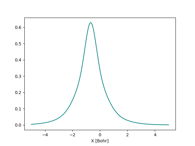
Let’s now plot the atomic orbitals and their overlap. We can do it by using the atomic_orbital() function, which evaluates the atomic orbital at a given coordinate. For instance, the value of the S orbital on the first hydrogen atom can be computed at the origin as

V1 = mol.atomic_orbital(0)
V1(0.0, 0.0, 0.0)

Out:

tensor(0.33796, requires_grad=True)

We can evaluate this orbital at different points along the \(x\) axis and plot it.

x = np.linspace(-5, 5, 1000)
plt.plot(x, V1(x, 0.0, 0.0), color='teal')
plt.xlabel('X [Bohr]')
plt.show()

We can also plot the second S orbital and visualize the overlap between them

V2 = mol.atomic_orbital(1)
plt.plot(x, V1(x, 0.0, 0.0), color='teal')
plt.plot(x, V2(x, 0.0, 0.0), color='teal')
plt.fill_between(
    x,  np.minimum(V1(x, 0.0, 0.0), V2(x, 0.0, 0.0)), color = 'red', alpha = 0.5, hatch = '||')
plt.xlabel('X [Bohr]')
plt.show()

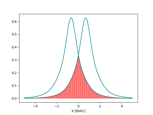
By looking at the orbitals, can you guess at what distance the value of the overlap becomes negligible? Can you verify your guess by computing the overlap at that distance?

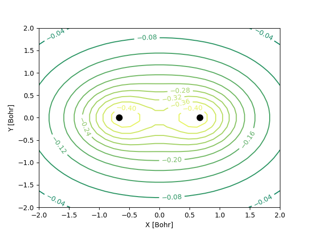
Similarly, we can plot the molecular orbitals of the hydrogen molecule obtained from the Hartree-Fock calculations. We plot the cross-section of the bonding orbital on the \(x-y\) plane.

n = 30 # number of grid points along each axis

mol.mo_coefficients = mol.mo_coefficients.T
mo = mol.molecular_orbital(0)
x, y = np.meshgrid(np.linspace(-2, 2, n),
                   np.linspace(-2, 2, n))
val = np.vectorize(mo)(x, y, 0)
val = np.array([val[i][j]._value for i in range(n) for j in range(n)]).reshape(n, n)

fig, ax = plt.subplots()
co = ax.contour(x, y, val, 10, cmap='summer_r', zorder=0)
ax.clabel(co, inline=2, fontsize=10)
plt.scatter(mol.coordinates[:,0], mol.coordinates[:,1], s = 80, color='black')
ax.set_xlabel('X [Bohr]')
ax.set_ylabel('Y [Bohr]')
plt.show()

VQE simulations

By performing the Hartree-Fock calculations, we obtain a set of one- and two-body integrals over molecular orbitals that can be used to construct the molecular Hamiltonian with the molecular_hamiltonian() function.

hamiltonian, qubits = qml.qchem.molecular_hamiltonian(mol.symbols,
                                                      mol.coordinates,
                                                      args=[mol.coordinates])
print(hamiltonian)

Out:

  (-0.2366648876198943) [Z2]
+ (-0.23666488761989424) [Z3]
+ (-0.05963862817464377) [I0]
+ (0.17575739479886338) [Z0]
+ (0.1757573947988635) [Z1]
+ (0.12222640951957497) [Z0 Z2]
+ (0.12222640951957497) [Z1 Z3]
+ (0.16714375519102576) [Z0 Z3]
+ (0.16714375519102576) [Z1 Z2]
+ (0.17001485407399825) [Z0 Z1]
+ (0.17570278345079388) [Z2 Z3]
+ (-0.04491734567145076) [Y0 Y1 X2 X3]
+ (-0.04491734567145076) [X0 X1 Y2 Y3]
+ (0.04491734567145076) [Y0 X1 X2 Y3]
+ (0.04491734567145076) [X0 Y1 Y2 X3]

The Hamiltonian contains 15 terms and, importantly, the coefficients of the Hamiltonian are all differentiable. We can construct a circuit and perform a VQE simulation in which both of the circuit parameters and the nuclear coordinates are optimized simultaneously by using the computed gradients. We will have two sets of differentiable parameters: the first set is the rotation angles of the excitation gates which are applied to the reference Hartree-Fock state to construct the exact ground state. The second set contains the nuclear coordinates of the hydrogen atoms.

dev = qml.device("default.qubit", wires=4)
def energy(mol):
    @qml.qnode(dev, interface="autograd")
    def circuit(*args):
        qml.BasisState(np.array([1, 1, 0, 0]), wires=range(4))
        qml.DoubleExcitation(*args[0][0], wires=[0, 1, 2, 3])
        H = qml.qchem.molecular_hamiltonian(mol.symbols, mol.coordinates, alpha=mol.alpha,
                                            coeff=mol.coeff, args=args[1:])[0]
        return qml.expval(H)
    return circuit

Note that we only use the DoubleExcitation gate as the SingleExcitation ones can be neglected in this particular example 2. We now compute the gradients of the energy with respect to the circuit parameter and the nuclear coordinates and update the parameters iteratively. Note that the nuclear coordinate gradients are simply the forces on the atomic nuclei.

# initial value of the circuit parameter
circuit_param = [np.array([0.0], requires_grad=True)]

for n in range(36):

    args = [circuit_param, geometry]
    mol = qml.qchem.Molecule(symbols, geometry)

    # gradient for circuit parameters
    g_param = grad(energy(mol), argnum = 0)(*args)
    circuit_param = circuit_param - 0.25 * g_param[0]

    # gradient for nuclear coordinates
    forces = -grad(energy(mol), argnum = 1)(*args)
    geometry = geometry + 0.5 * forces

    if n % 5 == 0:
        print(f'n: {n}, E: {energy(mol)(*args):.8f}, Force-max: {abs(forces).max():.8f}')

Out:

n: 0, E: -1.11750588, Force-max: 0.00001847
n: 5, E: -1.13514996, Force-max: 0.00410353
n: 10, E: -1.13704024, Force-max: 0.00210202
n: 15, E: -1.13727131, Force-max: 0.00084778
n: 20, E: -1.13730141, Force-max: 0.00032182
n: 25, E: -1.13730543, Force-max: 0.00011976
n: 30, E: -1.13730597, Force-max: 0.00004425
n: 35, E: -1.13730604, Force-max: 0.00001631

After 35 steps of optimization, the forces on the atomic nuclei and the gradient of the circuit parameter are both approaching zero, and the energy of the molecule is that of the optimized geometry at the full-CI level: \(-1.1373060483\) Ha. You can print the optimized geometry and verify that the final bond length of hydrogen is identical to the one computed with full-CI which is \(1.389\) Bohr.

We are now ready to perform a full optimization where the circuit parameters, the nuclear coordinates and the basis set parameters are all differentiable parameters that can be optimized simultaneously.

# initial values of the nuclear coordinates
geometry = np.array([[0.0, 0.0, -0.672943567415407],
                     [0.0, 0.0, 0.672943567415407]], requires_grad=True)

# initial values of the basis set exponents
alpha = np.array([[3.42525091, 0.62391373, 0.1688554],
                  [3.42525091, 0.62391373, 0.1688554]], requires_grad=True)

# initial values of the basis set contraction coefficients
coeff = np.array([[0.1543289673, 0.5353281423, 0.4446345422],
                  [0.1543289673, 0.5353281423, 0.4446345422]], requires_grad=True)

# initial value of the circuit parameter
circuit_param = [np.array([0.0], requires_grad=True)]

for n in range(36):

    args = [circuit_param, geometry, alpha, coeff]
    mol = qml.qchem.Molecule(symbols, geometry, alpha=alpha, coeff=coeff)

    # gradient for circuit parameters
    g_param = grad(energy(mol), argnum=0)(*args)
    circuit_param = circuit_param - 0.25 * g_param[0]

    # gradient for nuclear coordinates
    forces = -grad(energy(mol), argnum=1)(*args)
    geometry = geometry + 0.5 * forces

    # gradient for basis set exponents
    g_alpha = grad(energy(mol), argnum=2)(*args)
    alpha = alpha - 0.25 * g_alpha

    # gradient for basis set contraction coefficients
    g_coeff = grad(energy(mol), argnum=3)(*args)
    coeff = coeff - 0.25 * g_coeff

    if n % 5 == 0:
        print(f'n: {n}, E: {energy(mol)(*args):.8f}, Force-max: {abs(forces).max():.8f}')

Out:

n: 0, E: -1.11750589, Force-max: 0.00001847
n: 5, E: -1.13767645, Force-max: 0.00608084
n: 10, E: -1.13994674, Force-max: 0.00300161
n: 15, E: -1.14030200, Force-max: 0.00147246
n: 20, E: -1.14036879, Force-max: 0.00068656
n: 25, E: -1.14038648, Force-max: 0.00031174
n: 30, E: -1.14039502, Force-max: 0.00013847
n: 35, E: -1.14040160, Force-max: 0.00005926

You can also print the gradients of the circuit and basis set parameters and confirm that they are approaching zero. The computed energy of \(-1.14040160\) Ha is lower than the full-CI energy, \(-1.1373060483\) Ha (obtained with the STO-3G basis set for the hydrogen molecule) because we have optimized the basis set parameters in our example. This means that we can reach a lower energy for hydrogen without increasing the basis set size, which would otherwise lead to a larger number of qubits.

Conclusions

This tutorial introduces an important feature of PennyLane that allows performing fully-differentiable Hartree-Fock and subsequently VQE simulations. This feature provides two major benefits: i) All gradient computations needed for parameter optimization can be carried out with the elegant methods of automatic differentiation which facilitates simultaneous optimizations of circuit and Hamiltonian parameters in applications such as VQE molecular geometry optimizations. ii) By optimizing the molecular parameters such as the exponent and contraction coefficients of Gaussian functions of the basis set, one can reach a lower energy without increasing the number of basis functions. Can you think of other interesting molecular parameters that can be optimized along with the nuclear coordinates and basis set parameters that we optimized in this tutorial?

References

1(1,2,3)

Juan Miguel Arrazola, Soran Jahangiri, Alain Delgado, Jack Ceroni et al., “Differentiable quantum computational chemistry with PennyLane”. arXiv:2111.09967

2

Attila Szabo, Neil S. Ostlund, “Modern Quantum Chemistry: Introduction to Advanced Electronic Structure Theory”. Dover Publications, 1996.

About the author

Soran Jahangiri

Soran Jahangiri is a quantum chemist working at Xanadu. His work is focused on developing and implementing quantum algorithms for chemistry applications.

demos/tutorial_differentiable_HF

 

Download Python script

 

Download Notebook

 

View on GitHub