Givens rotations for quantum chemistry

Author: Juan Miguel Arrazola — Posted: 30 June 2021. Last updated: 30 June 2021.

In the book “Sophie’s world”, the young protagonist receives a white envelope containing a letter with an intriguing question: “Why is Lego the most ingenious toy in the world?” At first baffled by this curious message, she decides to reflect on the question. As told by the book’s narrator, she arrives at a conclusion:

The best thing about them was that with Lego she could construct any kind of object. And then she could separate the blocks and construct something new. What more could one ask of a toy? Sophie decided that Lego really could be called the most ingenious toy in the world.

In this tutorial, you will learn about the building blocks of quantum circuits for quantum chemistry: Givens rotations. These are operations that can be used to construct any kind of particle-conserving circuit. We discuss single and double excitation gates, which are particular types of Givens rotations that play an important role in quantum chemistry. Notably, controlled single excitation gates are universal for particle-conserving unitaries. You will also learn how to use these gates to build arbitrary states of a fixed number of particles.

Particle-conserving unitaries

Understanding the electronic structure of molecules is arguably the central problem in quantum chemistry. Quantum computers tackle this problem by using systems of qubits to represent the quantum states of the electrons. One method is to consider a collection of molecular orbitals, which capture the three-dimensional region of space occupied by the electrons. Each orbital can be occupied by at most two electrons, each with a different spin orientation. In this case we refer to spin orbitals that can be occupied by a single electron.

The state of electrons in a molecule can then be described by specifying how the orbitals are occupied. The Jordan-Wigner representation provides a convenient way to do this: we associate a qubit with each spin orbital and use its states to represent occupied \(|1\rangle\) or unoccupied \(|0\rangle\) spin orbitals.

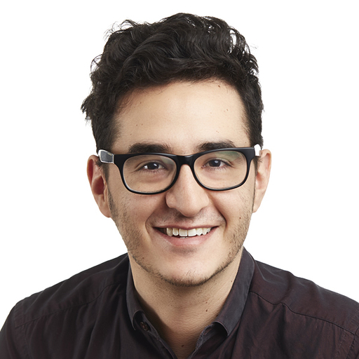
An \(n\)-qubit state with Hamming weight \(k\), i.e., with \(k\) qubits in state \(|1\rangle\), represents a state of \(k\) electrons in \(n\) spin orbitals. For example \(|1010\rangle\) is a state of two electrons in two spin orbitals. More generally, superpositions over all basis states with a fixed number of particles are valid states of the electrons in a molecule. These are states such as

\[|\psi\rangle = c_1|1100\rangle + c_2|1010\rangle + c_3|1001\rangle + c_4|0110\rangle + c_5|0101\rangle + c_6|0011\rangle,\]

for some coefficients \(c_i\).

States of a system with six spin orbitals and three electrons. Orbitals are for illustration; they correspond to carbon dioxide, which has more electrons and orbitals.

Because the number of electrons in a molecule is fixed, any transformation must conserve the number of particles. We refer to these as particle-conserving unitaries. When designing quantum circuits and algorithms for quantum chemistry, it is desirable to employ only particle-conserving gates that guarantee that the states of the system remain valid. This raises the questions: what are the simplest particle-conserving unitaries? Like Legos, how can they be used to construct any quantum circuit for quantum chemistry applications?

Givens rotations

Consider single-qubit gates. In their most general form, they perform the transformation

\[\begin{split}U|0\rangle &= a |0\rangle + b |1\rangle,\\ U|1\rangle &= c |1\rangle + d |0\rangle,\end{split}\]

where \(|a|^2+|b|^2=|c|^2+|d|^2=1\) and \(ab^* + cd^*=0\). This gate is particle-conserving only if \(b=d=0\), which means that the only single-qubit gates that preserve particle number are diagonal gates of the form

\[\begin{split}U = \begin{pmatrix} e^{i\theta} & 0\\ 0 & e^{i\phi} \end{pmatrix}.\end{split}\]

On their own, these gates are not very interesting. They can only be used to change the relative phases of states in a superposition; they cannot be used to create and control such superpositions. So let’s take a look at two-qubit gates.

Basis states of two qubits can be categorized depending on their number of particles.

We have:

• \(|00\rangle\) with zero particles,

• \(|01\rangle,|10\rangle\) with one particle, and

• \(|11\rangle\) with two particles.

We can now consider transformations that couple the states \(|01\rangle,|10\rangle\). These are gates of the form

\[\begin{split}U|01\rangle &= a |01\rangle + b |10\rangle\\ U|10\rangle &= c |10\rangle + d |01\rangle.\end{split}\]

This should be familiar: the unitary has the same form as a single-qubit gate, except that the states \(|01\rangle, |10\rangle\) respectively take the place of \(|0\rangle, |1\rangle\). This correspondence has a name: the dual-rail qubit, where a two-level system is constructed by specifying in which of two possible systems a single particle is located. The difference compared to single-qubit gates is that any values of the parameters \(a, b,c,d\) give rise to a valid particle-conserving unitary. Take for instance the two-qubit gate

\[\begin{split}G(\theta)=\begin{pmatrix} 1 & 0 & 0 & 0\\ 0 & \cos (\theta/2) & -\sin (\theta/2) & 0\\ 0 & \sin(\theta/2) & \cos(\theta/2) & 0\\ 0 & 0 & 0 & 1 \end{pmatrix}.\end{split}\]

This is an example of a Givens rotation: a rotation in a two-dimensional subspace of a larger Hilbert space. In this case, we are performing a Givens rotation in a two-dimensional subspace of the four-dimensional space of two-qubit states. This gate allows us to create superpositions by exchanging the particle between the two qubits. Such transformations can be interpreted as a single excitation, where we view the exchange from \(|10\rangle\) to \(|01\rangle\) as exciting the electron from the first to the second qubit.

A Givens rotation can be used to couple states that differ by a single excitation.

This gate is implemented in PennyLane as the SingleExcitation operation. We can use it to prepare an equal superposition of three-qubit states with a single particle \(\frac{1}{\sqrt{3}}(|001\rangle + |010\rangle + |100\rangle)\). We apply two single excitation gates with parameters \(\theta, \phi\) to the initial state \(|100\rangle\). The excitation gates act on qubits 0,1 and 0,2 respectively. This yields the state

\[|\psi\rangle = \cos(\theta/2)\cos(\phi/2)|100\rangle - \sin(\theta/2)|010\rangle - \cos(\theta/2)\sin(\phi/2)|001\rangle.\]

Since the amplitude of \(|010\rangle\) must be \(1/\sqrt{3}\), we conclude that \(-\sin(\theta/2)=1/\sqrt{3}\). This in turn implies that \(\cos(\theta/2)=\sqrt{2/3}\) and therefore \(-\sin(\phi/2)=1/\sqrt{2}\). Thus, to prepare an equal superposition state we choose the angles of rotation to be

\[\begin{split}\theta &= - 2 \arcsin(1/\sqrt{3}),\\ \phi &= - 2 \arcsin(1/\sqrt{2}).\end{split}\]

This can be implemented in PennyLane as follows:

import pennylane as qml
import numpy as np

dev = qml.device('default.qubit', wires=3)

@qml.qnode(dev, interface="autograd")
def circuit(x, y):
    # prepares the reference state |100>
    qml.BasisState(np.array([1, 0, 0]), wires=[0, 1, 2])
    # applies the single excitations
    qml.SingleExcitation(x, wires=[0, 1])
    qml.SingleExcitation(y, wires=[0, 2])
    return qml.state()

x = -2 * np.arcsin(np.sqrt(1/3))
y = -2 * np.arcsin(np.sqrt(1/2))
print(circuit(x, y))

Out:

[0.        +0.j 0.57735027+0.j 0.57735027+0.j 0.        +0.j
 0.57735027+0.j 0.        +0.j 0.        +0.j 0.        +0.j]

The components of the output state are ordered according to their binary representation, so entry 1 is \(|001\rangle\), entry 2 is \(|010\rangle\), and entry 4 is \(|100\rangle\), meaning we indeed prepared the desired state. We can check this by reshaping the output state

tensor_state = circuit(x, y).reshape(2, 2, 2)
print("Amplitude of state |001> = ", tensor_state[0, 0, 1])
print("Amplitude of state |010> = ", tensor_state[0, 1, 0])
print("Amplitude of state |100> = ", tensor_state[1, 0, 0])

Out:

Amplitude of state |001> =  (0.5773502691896258+0j)
Amplitude of state |010> =  (0.5773502691896256+0j)
Amplitude of state |100> =  (0.577350269189626+0j)

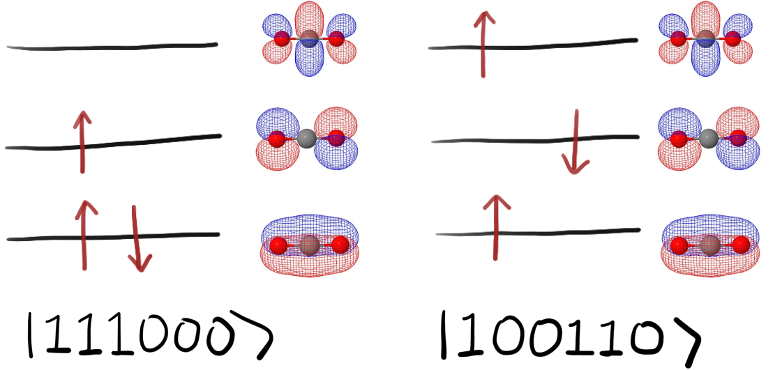
We can also study double excitations involving the transfer of two particles. For example, consider a Givens rotation in the subspace spanned by the states \(|1100\rangle\) and \(|0011\rangle\). These states differ by a double excitation since we can map \(|1100\rangle\) to \(|0011\rangle\) by exciting the particles from the first two qubits to the last two. Mathematically, this gate can be represented by a unitary \(G^{(2)}(\theta)\) that performs the mapping

\[\begin{split}G^{(2)}|0011\rangle &= \cos (\theta/2)|0011\rangle + \sin (\theta/2)|1100\rangle\\ G^{(2)}|1100\rangle &= \cos (\theta/2)|1100\rangle - \sin (\theta/2)|0011\rangle,\end{split}\]

while leaving all other basis states unchanged. This gate is implemented in PennyLane as the DoubleExcitation operation.

A Givens rotation can also be used to couple states that differ by a double excitation.

In the context of quantum chemistry, it is common to consider excitations on a fixed reference state and include only the excitations that preserve the spin orientation of the electron. For a system with \(n\) qubits and \(k\) particles, this reference state is typically chosen as the state with the first \(k\) qubits in state \(|1\rangle\), and the remainder in state \(|0\rangle\). PennyLane allows you to obtain all such excitations using the function excitations(). Let’s employ it to build a circuit that includes all single and double excitations acting on a reference state of three particles in six qubits. We apply a random rotation for each gate:

nr_particles = 3
nr_qubits = 6

singles, doubles = qml.qchem.excitations(3, 6)
print(f"Single excitations = {singles}")
print(f"Double excitations = {doubles}")

Out:

Single excitations = [[0, 4], [1, 3], [1, 5], [2, 4]]
Double excitations = [[0, 1, 3, 4], [0, 1, 4, 5], [1, 2, 3, 4], [1, 2, 4, 5]]

Now we continue to build the circuit:

dev2 = qml.device('default.qubit', wires=6)

@qml.qnode(dev2, interface="autograd")
def circuit2(x, y):
    # prepares reference state
    qml.BasisState(np.array([1, 1, 1, 0, 0, 0]), wires=[0, 1, 2, 3, 4, 5])
    # apply all single excitations
    for i, s in enumerate(singles):
        qml.SingleExcitation(x[i], wires=s)
    # apply all double excitations
    for j, d in enumerate(doubles):
        qml.DoubleExcitation(y[j], wires=d)
    return qml.state()

# random angles of rotation
x = np.random.normal(0, 1, len(singles))
y = np.random.normal(0, 1, len(doubles))

output = circuit2(x, y)

We can check which basis states appear in the resulting superposition to confirm that they involve only states with three particles.

# constructs binary representation of states with non-zero amplitude
states = [np.binary_repr(i, width=6) for i in range(len(output)) if output[i] != 0]
print(states)

Out:

['001011', '001110', '011010', '100011', '100110', '101001', '101100', '110010', '111000']

Besides these Givens rotations, there are other versions that have been reported in the literature and used to construct circuits for quantum chemistry. For instance, Ref. 1 considers a different sign convention for single-excitation gates,

\[\begin{split}G(\theta)=\begin{pmatrix} 1 & 0 & 0 & 0\\ 0 & \cos (\theta/2) & \sin (\theta/2) & 0\\ 0 & -\sin(\theta/2) & \cos(\theta/2) & 0\\ 0 & 0 & 0 & 1 \end{pmatrix},\end{split}\]

and Ref. 2 introduces the particle-conserving gates listed below, which are all Givens rotations

\[ \begin{align}\begin{aligned}\begin{split}U_1(\theta, \phi) &= \begin{pmatrix} 1 & 0 & 0 & 0\\ 0 & \cos (\theta) & e^{i\phi}\sin (\theta) & 0\\ 0 & e^{-i\phi}\sin(\theta) & -\cos(\theta) & 0\\ 0 & 0 & 0 & 1 \end{pmatrix},\\[12pt]\end{split}\\\begin{split}U_2(\theta) &= \begin{pmatrix} 1 & 0 & 0 & 0\\ 0 & \cos (2\theta) & -i\sin (2\theta) & 0\\ 0 & -i\sin(2\theta) & \cos(2\theta) & 0\\ 0 & 0 & 0 & 1 \end{pmatrix}.\end{split}\end{aligned}\end{align} \]

Givens rotations are a powerful abstraction for understanding quantum circuits for quantum chemistry. Instead of thinking of single-qubit gates and CNOTs as the building-blocks of quantum circuits, we can be more clever and select two-dimensional subspaces spanned by states with an equal number of particles, and use Givens rotations in that subspace to construct the circuits. 🧠

Controlled excitation gates

Single-qubit gates and CNOT gates are universal for quantum computing: they can be used to implement any conceivable quantum computation. If Givens rotations are analogous to single-qubit gates, then controlled Givens rotations are analogous to two-qubit gates. In universality constructions, the ability to control operations based on the states of other qubits is essential, so for this reason it’s natural to study controlled Givens rotations. The simplest of these are controlled single-excitation gates, which are three-qubit gates that perform the mapping

\[\begin{split}CG(\theta) |101\rangle &= \cos (\theta/2)|101\rangle + \sin (\theta/2)|110\rangle,\\ CG(\theta) |110\rangle &= \cos (\theta/2)|110\rangle - \sin (\theta/2)|101\rangle,\end{split}\]

while leaving all other basis states unchanged. This gate only excites a particle from the second to third qubit, and vice versa, if the first (control) qubit is in state \(|1\rangle\). This is a useful property: as the name suggests, it provides us with better control over the transformations we want to apply. Suppose we aim to prepare the state

\[|\psi\rangle = \frac{1}{2}(|110000\rangle + |001100\rangle + |000011\rangle + |100100\rangle).\]

Some inspection is enough to see that the states \(|001100\rangle\) and \(|000011\rangle\) differ by a double excitation from the reference state \(|110000\rangle\). Meanwhile, the state \(|100100\rangle\) differs by a single excitation. It is thus tempting to think that applying two double-excitation gates and a single-excitation gate can be used to prepare the target state. It won’t work! Applying the single-excitation gate on qubits 1 and 3 will also lead to an undesired contribution for the state \(|011000\rangle\) through a coupling with \(|001100\rangle\). Let’s check that this is the case:

dev = qml.device('default.qubit', wires=6)

@qml.qnode(dev, interface="autograd")
def circuit3(x, y, z):
    qml.BasisState(np.array([1, 1, 0, 0, 0, 0]), wires=[i for i in range(6)])
    qml.DoubleExcitation(x, wires=[0, 1, 2, 3])
    qml.DoubleExcitation(y, wires=[0, 1, 4, 5])
    qml.SingleExcitation(z, wires=[1, 3])
    return qml.state()

x = -2 * np.arcsin(np.sqrt(1/4))
y = -2 * np.arcsin(np.sqrt(1/3))
z = -2 * np.arcsin(np.sqrt(1/2))

output = circuit3(x, y, z)
states = [np.binary_repr(i, width=6) for i in range(len(output)) if output[i] != 0]
print(states)

Out:

['000011', '001100', '011000', '100100', '110000']

Indeed, we have a non-zero coefficient for \(|011000\rangle\). To address this problem, we can instead apply the single-excitation gate controlled on the state of the first qubit. This ensures that there is no coupling with the state \(| 001100\rangle\) since here the first qubit is in state \(|0\rangle\). Let’s implement the circuit above, this time controlling on the state of the first qubit and verify that we can prepare the desired state. To perform the control, we use the ctrl() transform:

@qml.qnode(dev, interface="autograd")
def circuit4(x, y, z):
    qml.BasisState(np.array([1, 1, 0, 0, 0, 0]), wires=[i for i in range(6)])
    qml.DoubleExcitation(x, wires=[0, 1, 2, 3])
    qml.DoubleExcitation(y, wires=[0, 1, 4, 5])
    # single excitation controlled on qubit 0
    qml.ctrl(qml.SingleExcitation, control=0)(z, wires=[1, 3])
    return qml.state()

output = circuit4(x, y, z)
states = [np.binary_repr(i, width=6) for i in range(len(output)) if output[i] != 0]
print(states)

Out:

['000011', '001100', '100100', '110000']

It was proven in Ref. 3 that controlled single-excitation gates are universal for particle-conserving unitaries. With enough ingenuity, you can use these operations to construct any kind of circuit for quantum chemistry applications. What more could you ask from a gate?

State preparation

We can bring all these pieces together and implement a circuit capable of preparing four-qubit states of two particles with real coefficients. The main idea is that we can perform the construction one basis state at a time by applying a suitable excitation gate, which may need to be controlled.

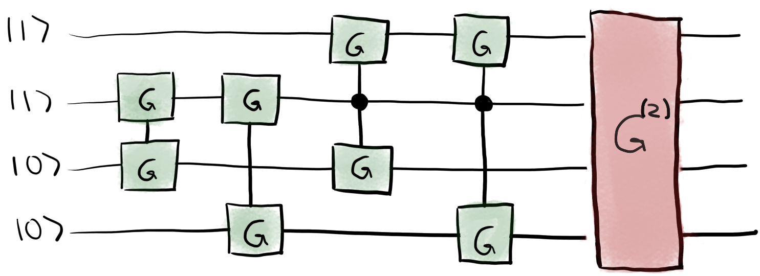
A circuit for preparing four-qubit states with two particles.

Starting from the reference state \(|1100\rangle\), we create a superposition with the state \(|1010\rangle\) by applying a single-excitation gate on qubits 1 and 2. Similarly, we create a superposition with the state \(|1001\rangle\) with a single excitation between qubits 1 and 3. This leaves us with a state of the form

\[|\psi\rangle = a |1100\rangle + b |1010\rangle + c |1001\rangle.\]

We can now perform two single excitations from qubit 0 to qubits 2 and 3. These will have to be controlled on the state of qubit 1. Finally, applying a double-excitation gate on all qubits can create a superposition of the form

\[|\psi\rangle = c_1|1100\rangle + c_2|1010\rangle + c_3|1001\rangle + c_4|0110\rangle + c_5|0101\rangle + c_6|0011\rangle,\]

which is our intended outcome. Let’s use this approach to create an equal superposition over all two-particle states on four qubits. We follow the same strategy as before, setting the angle of the \(k\)-th Givens rotation as \(-2 \arcsin(1/\sqrt{n-k})\), where \(n\) is the number of basis states in the superposition.

dev = qml.device('default.qubit', wires=4)

@qml.qnode(dev, interface="autograd")
def state_preparation(params):
    qml.BasisState(np.array([1, 1, 0, 0]), wires=[0, 1, 2, 3])
    qml.SingleExcitation(params[0], wires=[1, 2])
    qml.SingleExcitation(params[1], wires=[1, 3])
    # single excitations controlled on qubit 1
    qml.ctrl(qml.SingleExcitation, control=1)(params[2], wires=[0, 2])
    qml.ctrl(qml.SingleExcitation, control=1)(params[3], wires=[0, 3])
    qml.DoubleExcitation(params[4], wires=[0, 1, 2, 3])
    return qml.state()

n = 6
params = np.array([-2 * np.arcsin(1/np.sqrt(n-i)) for i in range(n-1)])

output = state_preparation(params)
# sets very small coefficients to zero
output[np.abs(output) < 1e-10] = 0
states = [np.binary_repr(i, width=4) for i in range(len(output)) if output[i] != 0]
print("Basis states = ", states)
print("Output state =", output)

Out:

Basis states =  ['0011', '0101', '0110', '1001', '1010', '1100']
Output state = [0.        +0.j 0.        +0.j 0.        +0.j 0.40824829+0.j
 0.        +0.j 0.40824829+0.j 0.40824829+0.j 0.        +0.j
 0.        +0.j 0.40824829+0.j 0.40824829+0.j 0.        +0.j
 0.40824829+0.j 0.        +0.j 0.        +0.j 0.        +0.j]

Success! This is the equal superposition state we wanted to prepare. 🚀

When it comes to quantum circuits for quantum chemistry, a wide variety of architectures have been proposed. Researchers in the field are faced with the apparent choice of making a selection among these circuits to conduct their computations and benchmark new algorithms. Like a kid in a toy store, it is challenging to pick just one.

Ultimately, the aim of this tutorial is to provide you with the conceptual and software tools to implement any of these proposed circuits, and also to design your own. It’s not only fun to play with toys; it’s also fun to build them.

References

1

G-L. R. Anselmetti, D. Wierichs, C. Gogolin, Christian, and R. M. Parrish, “Local, Expressive, Quantum-Number-Preserving VQE Ansatze for Fermionic Systems”, arXiv:2104.05695, (2021).

2

P. KL. Barkoutsos, Panagiotis, et al., “Quantum algorithms for electronic structure calculations: Particle-hole Hamiltonian and optimized wave-function expansions”, Physical Review A 98(2), 022322, (2018).

3

J. M. Arrazola, O. Di Matteo, N. Quesada, S. Jahangiri, A. Delgado, N. Killoran, “Universal quantum circuits for quantum chemistry”, arXiv:2106.13839, (2021)

About the author

Juan Miguel Arrazola

Juan Miguel is the Algorithms Senior Team Lead at Xanadu. His work focuses on developing quantum algorithms and related software for simulating molecules and materials.

demos/tutorial_givens_rotations

 

Download Python script

 

Download Notebook

 

View on GitHub