Doubly stochastic gradient descent

Author: Josh Izaac — Posted: 16 October 2019. Last updated: 20 January 2021.

In this tutorial we investigate and implement the doubly stochastic gradient descent paper from Ryan Sweke et al. (2019). In this paper, it is shown that quantum gradient descent, where a finite number of measurement samples (or shots) are used to estimate the gradient, is a form of stochastic gradient descent. Furthermore, if the optimization involves a linear combination of expectation values (such as VQE), sampling from the terms in this linear combination can further reduce required resources, allowing for “doubly stochastic gradient descent”.

Note that based on very similar observations, Jonas Kuebler et al. (2019) recently proposed an optimizer (which they call the individual Coupled Adaptive Number of Shots (iCANS) optimizer) that adapts the shot number of measurements during training.

Background

In classical machine learning, stochastic gradient descent is a common optimization strategy where the standard gradient descent parameter update rule,

\[\theta^{(t+1)} = \theta^{(t)} - \eta \nabla \mathcal{L}(\theta^{(t)}),\]

is modified such that

\[\theta^{(t+1)} = \theta^{(t)} - \eta g^{(t)}(\theta^{(t)})\]

where \(\eta\) is the step-size, and \(\{g^{(t)}(\theta)\}\) is a sequence of random variables such that

\[\mathbb{E}[g^{(t)}(\theta)] = \nabla\mathcal{L}(\theta).\]

In general, stochastic gradient descent is preferred over standard gradient descent for several reasons:

1. Samples of the gradient estimator \(g^{(t)}(\theta)\) can typically be computed much more efficiently than \(\mathcal{L}(\theta)\),

2. Stochasticity can help to avoid local minima and saddle points,

3. Numerical evidence shows that convergence properties are superior to regular gradient descent.

In variational quantum algorithms, a parametrized quantum circuit \(U(\theta)\) is optimized by a classical optimization loop in order to minimize a function of the expectation values. For example, consider the expectation values

\[\langle A_i \rangle = \langle 0 | U(\theta)^\dagger A_i U(\theta) | 0\rangle\]

for a set of observables \(\{A_i\}\), and loss function

\[\mathcal{L}(\theta, \langle A_1 \rangle, \dots, \langle A_M \rangle).\]

While the expectation values can be calculated analytically in classical simulations, on quantum hardware we are limited to sampling from the expectation values; as the number of samples (or shots) increase, we converge on the analytic expectation value, but can never recover the exact expression. Furthermore, the parameter-shift rule (Schuld et al., 2018) allows for analytic quantum gradients to be computed from a linear combination of the variational circuits’ expectation values.

Putting these two results together, Sweke et al. (2019) show that samples of the expectation value fed into the parameter-shift rule provide unbiased estimators of the quantum gradient—resulting in a form of stochastic gradient descent (referred to as QSGD). Moreover, they show that convergence of the stochastic gradient descent is guaranteed in sufficiently simplified settings, even in the case where the number of shots is 1!

Note

It is worth noting that the smaller the number of shots used, the larger the variance in the estimated expectation value. As a result, it may take more optimization steps for convergence than using a larger number of shots, or an exact value.

At the same time, a reduced number of shots may significantly reduce the wall time of each optimization step, leading to a reduction in the overall optimization time.

Let’s consider a simple example in PennyLane, comparing analytic gradient descent (with exact expectation values) to stochastic gradient descent using a finite number of shots.

A single-shot stochastic gradient descent

Consider the Hamiltonian

\[\begin{split}H = \begin{bmatrix} 8 & 4 & 0 & -6\\ 4 & 0 & 4 & 0\\ 0 & 4 & 8 & 0\\ -6 & 0 & 0 & 0 \end{bmatrix}.\end{split}\]

We can solve for the ground state energy using the variational quantum eigensolver (VQE) algorithm.

Let’s use the default.qubit simulator for both the analytic gradient, as well as the estimated gradient using number of shots \(N\in\{1, 100\}\).

import pennylane as qml
from pennylane import numpy as np

np.random.seed(3)

from pennylane import expval
from pennylane.templates.layers import StronglyEntanglingLayers

num_layers = 2
num_wires = 2
eta = 0.01
steps = 200

dev_analytic = qml.device("default.qubit", wires=num_wires, shots=None)
dev_stochastic = qml.device("default.qubit", wires=num_wires, shots=1000)

We can use qml.Hermitian to directly specify that we want to measure the expectation value of the matrix \(H\):

H = np.array([[8, 4, 0, -6], [4, 0, 4, 0], [0, 4, 8, 0], [-6, 0, 0, 0]], requires_grad=False)


def circuit(params):
    StronglyEntanglingLayers(weights=params, wires=[0, 1])
    return expval(qml.Hermitian(H, wires=[0, 1]))

Now, we create three QNodes, each corresponding to a device above, and optimize them using gradient descent via the parameter-shift rule.

qnode_analytic = qml.QNode(circuit, dev_analytic, interface="autograd")
qnode_stochastic = qml.QNode(circuit, dev_stochastic, interface="autograd")

param_shape = StronglyEntanglingLayers.shape(n_layers=num_layers, n_wires=num_wires)
init_params = np.random.uniform(low=0, high=2*np.pi, size=param_shape, requires_grad=True)

# Optimizing using exact gradient descent

cost_GD = []
params_GD = init_params
opt = qml.GradientDescentOptimizer(eta)

for _ in range(steps):
    cost_GD.append(qnode_analytic(params_GD))
    params_GD = opt.step(qnode_analytic, params_GD)

# Optimizing using stochastic gradient descent with shots=1

dev_stochastic.shots = 1
cost_SGD1 = []
params_SGD1 = init_params
opt = qml.GradientDescentOptimizer(eta)

for _ in range(steps):
    cost_SGD1.append(qnode_stochastic(params_SGD1))
    params_SGD1 = opt.step(qnode_stochastic, params_SGD1)

# Optimizing using stochastic gradient descent with shots=100

dev_stochastic.shots = 100
cost_SGD100 = []
params_SGD100 = init_params
opt = qml.GradientDescentOptimizer(eta)

for _ in range(steps):
    cost_SGD100.append(qnode_stochastic(params_SGD100))
    params_SGD100 = opt.step(qnode_stochastic, params_SGD100)

Note that in the latter two cases we are sampling from an unbiased estimator of the cost function, not the analytic cost function.

To track optimization convergence, approaches could include:

• Evaluating the cost function with a larger number of samples at specified intervals,

• Keeping track of the moving average of the low-shot cost evaluations.

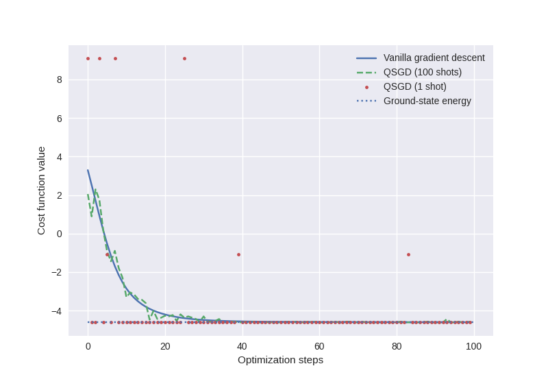
We can now plot the cost against optimization step for the three cases above.

from matplotlib import pyplot as plt

plt.style.use("seaborn")
plt.plot(cost_GD[:100], label="Vanilla gradient descent")
plt.plot(cost_SGD100[:100], "--", label="QSGD (100 shots)")
plt.plot(cost_SGD1[:100], ".", label="QSGD (1 shot)")

# analytic ground state
min_energy = min(np.linalg.eigvalsh(H))
plt.hlines(min_energy, 0, 100, linestyles=":", label="Ground-state energy")

plt.ylabel("Cost function value")
plt.xlabel("Optimization steps")
plt.legend()
plt.show()

Using the trained parameters from each optimization strategy, we can evaluate the analytic quantum device:

print("Vanilla gradient descent min energy = ", qnode_analytic(params_GD))
print(
    "Stochastic gradient descent (shots=100) min energy = ",
    qnode_analytic(params_SGD100),
)
print(
    "Stochastic gradient descent (shots=1) min energy = ", qnode_analytic(params_SGD1)
)

Out:

Vanilla gradient descent min energy =  -4.605247234069293
Stochastic gradient descent (shots=100) min energy =  -4.6006551769161455
Stochastic gradient descent (shots=1) min energy =  -4.457668962761632

Amazingly, we see that even the shots=1 optimization converged to a reasonably close approximation of the ground-state energy!

Doubly stochastic gradient descent for VQE

As noted in Sweke et al. (2019), variational quantum algorithms often include terms consisting of linear combinations of expectation values. This is true of the parameter-shift rule (where the gradient of each parameter is determined by shifting the parameter by macroscopic amounts and taking the difference), as well as VQE, where the Hamiltonian is usually decomposed into a sum of Pauli expectation values.

Consider the Hamiltonian from the previous section. As this Hamiltonian is a Hermitian observable, we can always express it as a sum of Pauli matrices using the relation

\[H = \sum_{i,j=0,1,2,3} a_{i,j} (\sigma_i\otimes \sigma_j),\]

where

\[a_{i,j} = \frac{1}{4}\text{tr}[(\sigma_i\otimes \sigma_j )H], ~~ \sigma = \{I, X, Y, Z\}.\]

Applying this, we can see that

\[H = 4 + 2I\otimes X + 4I \otimes Z - X\otimes X + 5 Y\otimes Y + 2Z\otimes X.\]

To perform “doubly stochastic” gradient descent, we simply apply the stochastic gradient descent approach from above, but in addition also uniformly sample a subset of the terms for the Hamiltonian expectation at each optimization step. This inserts another element of stochasticity into the system—all the while convergence continues to be guaranteed!

Let’s create a QNode that randomly samples a single term from the above Hamiltonian as the observable to be measured.

I = np.identity(2)
X = np.array([[0, 1], [1, 0]])
Y = np.array([[0, -1j], [1j, 0]])
Z = np.array([[1, 0], [0, -1]])

terms = np.array(
    [
        2 * np.kron(I, X),
        4 * np.kron(I, Z),
        -np.kron(X, X),
        5 * np.kron(Y, Y),
        2 * np.kron(Z, X),
    ], requires_grad=False
)


@qml.qnode(dev_stochastic, interface="autograd")
def circuit(params, n=None):
    StronglyEntanglingLayers(weights=params, wires=[0, 1])
    idx = np.random.choice(np.arange(5), size=n, replace=False)
    A = np.sum(terms[idx], axis=0)
    return expval(qml.Hermitian(A, wires=[0, 1]))


def loss(params):
    return 4 + (5 / 1) * circuit(params, n=1)

Optimizing the circuit using gradient descent via the parameter-shift rule:

dev_stochastic.shots = 100
cost = []
params = init_params
opt = qml.GradientDescentOptimizer(0.005)

for _ in range(250):
    cost.append(loss(params))
    params = opt.step(loss, params)

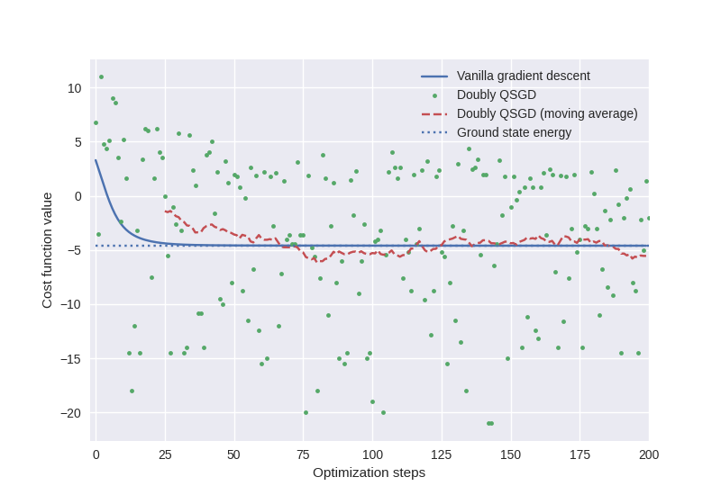
During doubly stochastic gradient descent, we are sampling from terms of the analytic cost function, so it is not entirely instructive to plot the cost versus optimization step—partial sums of the terms in the Hamiltonian may have minimum energy below the ground state energy of the total Hamiltonian. Nevertheless, we can keep track of the cost value moving average during doubly stochastic gradient descent as an indicator of convergence.

def moving_average(data, n=3):
    ret = np.cumsum(data, dtype=np.float64)
    ret[n:] = ret[n:] - ret[:-n]
    return ret[n - 1 :] / n


average = np.vstack([np.arange(25, 200), moving_average(cost, n=50)[:-26]])

plt.plot(cost_GD, label="Vanilla gradient descent")
plt.plot(cost, ".", label="Doubly QSGD")
plt.plot(average[0], average[1], "--", label="Doubly QSGD (moving average)")
plt.hlines(min_energy, 0, 200, linestyles=":", label="Ground state energy")

plt.ylabel("Cost function value")
plt.xlabel("Optimization steps")
plt.xlim(-2, 200)
plt.legend()
plt.show()

Finally, verifying that the doubly stochastic gradient descent optimization correctly provides the ground state energy when evaluated for a larger number of shots:

print("Doubly stochastic gradient descent min energy = ", qnode_analytic(params))

Out:

Doubly stochastic gradient descent min energy =  -4.499019593095161

While stochastic gradient descent requires more optimization steps to achieve convergence, it is worth noting that it requires significantly fewer quantum device evaluations, and thus may as a result take less time overall.

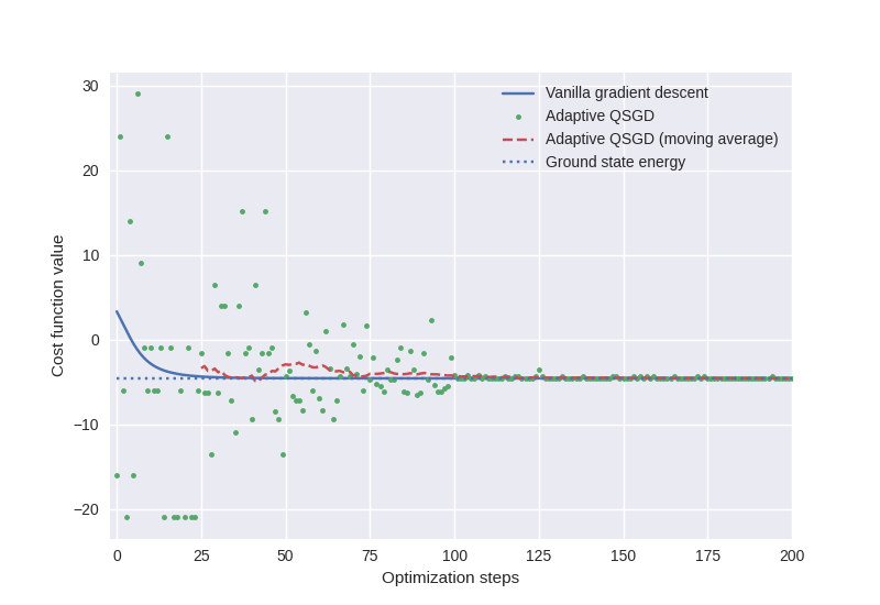
Adaptive stochasticity

To improve on the convergence, we may even consider a crude “adaptive” modification of the doubly stochastic gradient descent optimization performed above. In this approach, we successively increase the number of terms we are sampling from as the optimization proceeds, as well as increasing the number of shots.

cost = []
params = init_params
opt = qml.GradientDescentOptimizer(0.005)

for i in range(250):
    n = min(i // 25 + 1, 5)
    dev_stochastic.shots = int(1 + (n - 1) ** 2)

    def loss(params):
        return 4 + (5 / n) * circuit(params, n=n)

    cost.append(loss(params))
    params = opt.step(loss, params)

average = np.vstack([np.arange(25, 200), moving_average(cost, n=50)[:-26]])

plt.plot(cost_GD, label="Vanilla gradient descent")
plt.plot(cost, ".", label="Adaptive QSGD")
plt.plot(average[0], average[1], "--", label="Adaptive QSGD (moving average)")
plt.hlines(min_energy, 0, 250, linestyles=":", label="Ground state energy")

plt.ylabel("Cost function value")
plt.xlabel("Optimization steps")
plt.xlim(-2, 200)
plt.legend()
plt.show()

print("Adaptive QSGD min energy = ", qnode_analytic(params))

Out:

Adaptive QSGD min energy =  -4.592548741613163

References

1. Ryan Sweke, Frederik Wilde, Johannes Jakob Meyer, Maria Schuld, Paul K. Fährmann, Barthélémy Meynard-Piganeau, Jens Eisert. “Stochastic gradient descent for hybrid quantum-classical optimization.” arXiv:1910.01155, 2019.

About the author

Josh Izaac

Josh is a theoretical physicist, software tinkerer, and occasional baker. At Xanadu, he contributes to the development and growth of Xanadu’s open-source quantum software products.

demos/tutorial_doubly_stochastic

 

Download Python script

 

Download Notebook

 

View on GitHub