The stochastic parameter-shift rule

Author: Nathan Killoran — Posted: 25 May 2020. Last updated: 15 January 2021.

We demonstrate how the stochastic parameter-shift rule, discovered by Banchi and Crooks 1, can be used to differentiate arbitrary qubit gates, generalizing the original parameter-shift rule, which applies only for gates of a particular (but widely encountered) form.

Background

One of the main ideas encountered in near-term quantum machine learning is the variational circuit. Evolving from earlier concepts pioneered by domain-specific algorithms like the variational quantum eigensolver and the quantum approximate optimization algorithm, this class of quantum algorithms makes heavy use of two distinguishing ingredients:

1. The circuit’s gates have free parameters

2. Expectation values of measurements are built up from samples

These two ingredients allow one circuit to actually represent an entire family of circuits. An objective function—encapsulating some problem-specific goal—is built from the expectation values, and the circuit’s free parameters are progressively tuned to optimize this function. At each step, the circuit has the same gate layout, but slightly different parameters, making this approach promising to run on constrained near-term devices.

But how should we actually update the circuit’s parameters to move us closer to a good output? Borrowing a page from classical optimization and deep learning, we can use gradient descent. In this general-purpose method, we compute the derivative of a (smooth) function \(f\) with respect to its parameters \(\theta\), i.e., its gradient \(\nabla_\theta f\). Since the gradient always points in the direction of steepest ascent/descent, if we make small updates to the parameters according to

\[\theta \rightarrow \theta - \eta \nabla_\theta f,\]

we can iteratively progress to lower and lower values of the function.

The Parameter-Shift Rule

In the quantum case, the expectation value of a circuit with respect to an measurement operator \(\hat{C}\) depends smoothly on the the circuit’s gate parameters \(\theta\). We can write this expectation value as \(\langle \hat{C}(\theta)\rangle\). This means that the derivatives \(\nabla_\theta \langle \hat{C} \rangle\) exist and gradient descent can be used.

Before digging deeper, we will first set establish some basic notation. For simplicity, though a circuit may contain many gates, we can concentrate on just a single gate \(\hat{U}\) that we want to differentiate (other gates will follow the same pattern).

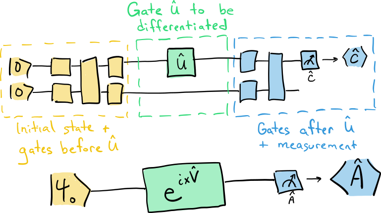
All gates appearing before \(\hat{U}\) can be absorbed into an initial state preparation \(\vert \psi_0 \rangle\), and all gates appearing after \(\hat{U}\) can be absorbed with the measurement operator \(\hat{C}\) to make a new effective measurement operator \(\hat{A}\). The expectation value \(\hat{A}\) in the simpler one-gate circuit is identical to the expectation value \(\hat{C}\) in the larger circuit.

We can also write any unitary gate in the form

\[\hat{U}(\theta) = e^{i\theta\hat{V}},\]

where \(\hat{V}\) is the Hermitian generator of the gate \(\hat{U}\).

Now, how do we actually obtain the numerical values of the gradient necessary for gradient descent?

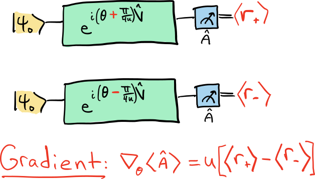
This is where the parameter-shift rule 2 3 4 enters the story. In short, the parameter-shift rule says that for many gates of interest—including all single-qubit gates—we can obtain the value of the derivative \(\nabla_\theta \langle \hat{A}(\theta) \rangle\) by subtracting two related circuit evaluations:

\[\nabla_\theta \langle \hat{A} \rangle = u\left[ \langle \hat{A}(\theta + \tfrac{\pi}{4u}) \rangle - \langle \hat{A}(\theta - \tfrac{\pi}{4u}) \rangle \right]\]

Note

The multiplier \(u\) in this formula is arbitrary and can differ between implementations. For example, PennyLane internally uses the convention where \(u=\tfrac{1}{2}\).

The parameter-shift rule is exact, i.e., the formula for the gradient doesn’t involve any approximations. For quantum hardware, we can only take a finite number of samples, so we can never determine a circuit’s expectation values exactly. However, the parameter-shift rule provides the guarantee that it is an unbiased estimator, meaning that if we could take a infinite number of samples, it converges to the correct gradient value.

Let’s jump into some code and take a look at the parameter-shift rule in action.

import pennylane as qml
import matplotlib.pyplot as plt
from pennylane import numpy as np
from scipy.linalg import expm

np.random.seed(143)
angles = np.linspace(0, 2 * np.pi, 50)
dev = qml.device('default.qubit', wires=2)

We will consider a very simple circuit, containing just a single-qubit rotation about the x-axis, followed by a measurement along the z-axis.

@qml.qnode(dev)
def rotation_circuit(theta):
    qml.RX(theta, wires=0)
    return qml.expval(qml.PauliZ(0))

We will examine the gradient with respect to the parameter \(\theta\). The parameter-shift recipe requires taking the difference of two circuit evaluations, with forward and backward shifts in angles. PennyLane also provides a convenience function grad() to automatically compute the gradient. We can use it here for comparison.

Note

Check out the qml.gradients module to explore all quantum gradient transforms provided by PennyLane.

def param_shift(theta):
    # using the convention u=1/2
    r_plus = rotation_circuit(theta + np.pi / 2)
    r_minus = rotation_circuit(theta - np.pi / 2)
    return 0.5 * (r_plus - r_minus)

gradient = qml.grad(rotation_circuit, argnum=0)

expvals = [rotation_circuit(theta) for theta in angles]
grad_vals = [gradient(theta) for theta in angles]
param_shift_vals = [param_shift(theta) for theta in angles]
plt.plot(angles, expvals, 'b', label="Expecation value")
plt.plot(angles, grad_vals, 'r', label="qml.grad function")
plt.plot(angles, param_shift_vals, 'mx', label="Parameter-shift rule")
plt.xlabel("theta")
plt.legend()
plt.show()

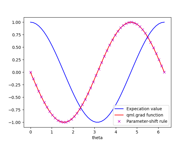
We have evaluated the expectation value at all possible values for the angle \(\theta\). By inspection, we can see that the functional dependence is \(\cos(\theta)\).

The parameter-shift evaluations are plotted with ‘x’ markers. Again, by simple inspection, we can see that these have the functional form \(-\sin(\theta)\), the expected derivative of \(\cos(\theta)\), and that they match the values provided by the grad() function.

The parameter-shift works really nicely for many gates—like the rotation gate we used in our example above. But it does have constraints. There are some technical conditions that, if a gate satisfies them, we can guarantee it has a parameter-shift rule 4. Concretely, the parameter-shift rule holds for any gate of the form \(e^{i\theta\hat{G}}\) where \(\hat{G}^2=\mathbb{1}\). Furthermore, we can derive similar parameter-shift recipes for some other gates that don’t meet this technical conditions, on a one-by-one basis.

But, in general, the parameter-shift rule is not universally applicable. In cases where it does not hold (or is not yet known to hold), we would either have to decompose the gate into compatible gates, or use an alternate estimator for the gradient, e.g., the finite-difference approximation. But both of these alternatives can have drawbacks due to increased circuit complexity or potential errors in the gradient value.

If only there was a parameter-shift method that could be used for any qubit gate. 🤔

The Stochastic Parameter-Shift Rule

Here’s where the stochastic parameter-shift rule makes its appearance on the stage.

The stochastic parameter-shift rule introduces two new ingredients to the parameter-shift recipe:

1. A random parameter \(s\), sampled uniformly from \([0,1]\) (this is the origin of the “stochastic” in the name);

2. Sandwiching the “shifted” gate application with one additional gate on each side.

These additions allow the stochastic parameter-shift rule to work for arbitrary qubit gates.

Every gate is unitary, which means they have the form \(\hat{U}(\theta) = e^{i\theta \hat{G}}\) for some generator \(G\). Additionally, every multi-qubit operator can be expressed as a sum of tensor products of Pauli operators, so let’s assume, without loss of generality, the following form for \(\hat{G}\):

\[\hat{G} = \hat{H} + \theta \hat{V},\]

where \(\hat{V}\) is a “Pauli word”, i.e., a tensor product of Pauli operators (e.g., \(\hat{Z}_0\otimes\hat{Y}_1)\) and \(\hat{H}\) can be an arbitrary linear combination of Pauli-operator tensor products. For simplicity, we assume that the parameter \(\theta\) appears only in front of \(\hat{V}\) (other cases can be handled using the chain rule).

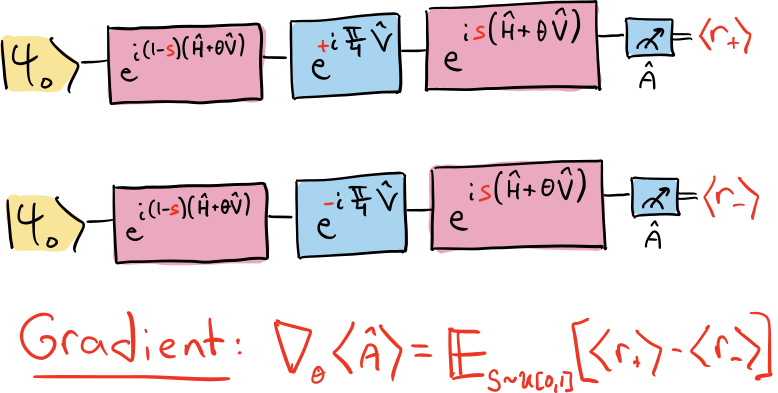
The stochastic parameter-shift rule gives the following recipe for computing the gradient of the expectation value \(\langle \hat{A} (\theta) \rangle\):

1. Sample a value for the variable \(s\) uniformly form \([0,1]\).

2. In place of gate \(\hat{U}(\theta)\), apply the following three gates:

   1. \(e^{i(1-s)(\hat{H} + \theta\hat{V})}\)

   2. \(e^{+i\tfrac{\pi}{4}\hat{V}}\)

   3. \(e^{is(\hat{H} + \theta\hat{V})}\)

   Measure the observable \(\hat{A}\) and call the resulting expectation value of \(\langle r_+\rangle\).

3. Repeat step ii, but flip the sign of the angle \(\tfrac{\pi}{4}\) in part b. Call the resulting expectation value \(\langle r_-\rangle\).

The gradient can be obtained from the average value of \(\langle r_+ \rangle - \langle r_-\rangle\), i.e.,

\[\mathbb{E}_{s\in\mathcal{U}[0,1]}[\langle r_+ \rangle - \langle r_-\rangle]\]

Let’s see this method in action.

Following 1, we will use the cross-resonance gate as a working example. This gate is defined as

\[\hat{U}_{CR}(\theta_1, \theta_2, \theta_3) = \exp\left[ i(\theta_1\hat{X}\otimes\hat{\mathbf{1}} - \theta_2\hat{Z}\otimes\hat{X} + \theta_3\hat{\mathbf{1}}\otimes\hat{X} ) \right].\]

# First we define some basic Pauli matrices
I = np.eye(2)
X = np.array([[0, 1], [1, 0]])
Z = np.array([[1, 0], [0, -1]])

def Generator(theta1, theta2, theta3):
    G = theta1.item() * np.kron(X, I) - \
        theta2 * np.kron(Z, X) + \
        theta3 * np.kron(I, X)
    return G

# A simple example circuit that contains the cross-resonance gate
@qml.qnode(dev)
def crossres_circuit(gate_pars):
    G = Generator(*gate_pars)
    qml.QubitUnitary(expm(-1j * G), wires=[0, 1])
    return qml.expval(qml.PauliZ(0))

# Subcircuit implementing the gates necessary for the
# stochastic parameter-shift rule.
# In this example, we will differentiate the first term of
# the circuit (i.e., our variable is theta1).
def SPSRgates(gate_pars, s, sign):
    G = Generator(*gate_pars)
    # step a)
    qml.QubitUnitary(expm(1j * (1 - s) * G), wires=[0, 1])
    # step b)
    qml.QubitUnitary(expm(1j * sign * np.pi / 4 * X), wires=0)
    # step c)
    qml.QubitUnitary(expm(1j * s * G), wires=[0,1])

# Function which can obtain all expectation vals needed
# for the stochastic parameter-shift rule
@qml.qnode(dev)
def spsr_circuit(gate_pars, s=None, sign=+1):
    SPSRgates(gate_pars, s, sign)
    return qml.expval(qml.PauliZ(0))

# Fix the other parameters of the gate
theta2, theta3 = -0.15, 1.6

# Obtain r+ and r-
# Even 10 samples gives a good result for this example
pos_vals = np.array([[spsr_circuit([theta1, theta2, theta3], s=s, sign=+1)
                      for s in np.random.uniform(size=10)]
                      for theta1 in angles])
neg_vals = np.array([[spsr_circuit([theta1, theta2, theta3], s=s, sign=-1)
                      for s in np.random.uniform(size=10)]
                      for theta1 in angles])

# Plot the results
evals = [crossres_circuit([theta1, theta2, theta3]) for theta1 in angles]
spsr_vals = (pos_vals - neg_vals).mean(axis=1)
plt.plot(angles, evals, 'b', label="Expectation Value")
plt.plot(angles, spsr_vals, 'r', label="Stochastic parameter-shift rule")
plt.xlabel("theta1")
plt.legend()
plt.show()

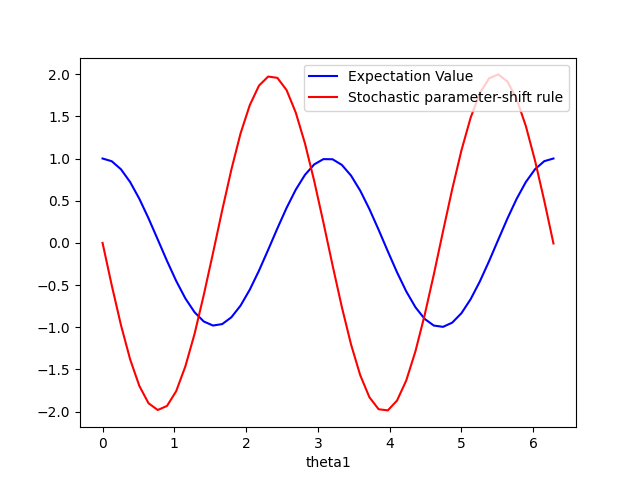
By inspection, we can see that the expectation values of the cross-resonance gate lead to a functional form \(\cos(2\theta_1)\). Also by inspection, the results from the stochastic parameter-shift rule have the functional form \(-2\sin(2\theta_1)\), which is the derivative of \(\cos(2\theta_1)\)!

Finally, it is interesting to notice when the stochastic parameter-shift rule reduces to the regular parameter-shift rule. Consider again the case where the gate has just a single term:

\[\hat{U}(\theta) = e^{i\theta\hat{V}}.\]

In this case, the terms encapsulated in the operator \(\hat{H}\) are all zero, and the gates \(e^{i(1-s)\hat{G}}\), \(e^{\pm i\tfrac{\pi}{4}\hat{V}}\), and \(e^{is\hat{G}}\) which appear in the stochastic parameter-shift rule all commute. Therefore, we can combine them together into a single gate:

\[\begin{split}\begin{align} e^{i(1-s)\hat{G}}e^{\pm i\tfrac{\pi}{4}\hat{V}}e^{is\hat{G}} & = e^{i(1-s)\hat{G}}e^{is\hat{G}}e^{\pm i\tfrac{\pi}{4}\hat{V}} \\ & = e^{i\hat{G}}e^{\pm i\tfrac{\pi}{4}\hat{V}} \\ & = e^{i\theta\hat{V}}e^{\pm i\tfrac{\pi}{4}\hat{V}} \\ & = e^{i\left(\theta\pm\tfrac{\pi}{4}\right)\hat{V}} \end{align}\end{split}\]

Since the random variable \(s\) no longer appears in this equation, averaging over it has no effect, and the stochastic parameter-shift rule nicely reduces back to the ordinary parameter-shift rule!

\[\begin{align} \mathbb{E}_{s\in\mathcal{U}[0,1]}\left[ e^{i(1-s)\hat{G}}e^{\pm i\tfrac{\pi}{4}\hat{V}}e^{is\hat{G}} \right] = & e^{i\left(\theta\pm\tfrac{\pi}{4}\right)\hat{V}} \end{align}\]

References

1(1,2)

Leonardo Banchi and Gavin E. Crooks. “Measuring Analytic Gradients of General Quantum Evolution with the Stochastic Parameter Shift Rule.” Quantum **5** 386 (2021).

2

Jun Li, Xiaodong Yang, Xinhua Peng, and Chang-Pu Sun. “Hybrid Quantum-Classical Approach to Quantum Optimal Control.” arXiv:1608.00677 (2016).

3

Kosuke Mitarai, Makoto Negoro, Masahiro Kitagawa, and Keisuke Fujii. “Quantum Circuit Learning.” arXiv:1803.00745 (2020).

4(1,2)

Maria Schuld, Ville Bergholm, Christian Gogolin, Josh Izaac, and Nathan Killoran. “Evaluating analytic gradients on quantum hardware.” arXiv:1811.11184 (2019).

About the author

Nathan Killoran

Nathan is the Chief Technical Officer—Software at Xanadu. You might recognize him from his work on PennyLane, quantum machine learning, and founding the famous QHack Meme Contest.

demos/tutorial_stochastic_parameter_shift

 

Download Python script

 

Download Notebook

 

View on GitHub