Generalized parameter-shift rules

Author: David Wierichs (Xanadu Resident) — Posted: 23 August 2021. Last updated: 27 August 2021

In this demo we will look at univariate quantum functions, i.e., those that depend on a single parameter. We will investigate the form such functions usually take and demonstrate how we can reconstruct them as classical functions, capturing the full dependence on the input parameter. Once we have this reconstruction, we use it to compute analytically exact derivatives of the quantum function. We implement this in two ways: first, by using autodifferentiation on the classical function that is produced by the reconstruction, which is flexible with respect to the degree of the derivative. Second, by computing the derivative manually, resulting in generalized parameter-shift rules for quantum functions that is more efficient (regarding classical cost) than the autodifferentiation approach, but requires manual computations if we want to access higher-order derivatives. All we will need for the demo is the insight that these functions are Fourier series in their variable, and the reconstruction itself is a trigonometric interpolation.

A full description of the reconstruction, the technical derivation of the parameter-shift rules, and considerations for multivariate functions can be found in the paper General parameter-shift rules for quantum gradients 1. The core idea to consider these quantum functions as Fourier series was first presented in the preprint Calculus on parameterized quantum circuits 2. We will follow 1, but there also are two preprints discussing general parameter-shift rules: an algebraic approach in Analytic gradients in variational quantum algorithms: Algebraic extensions of the parameter-shift rule to general unitary transformations 4 and one focusing on special gates and spectral decompositions, namely Generalized quantum circuit differentiation rules 5.

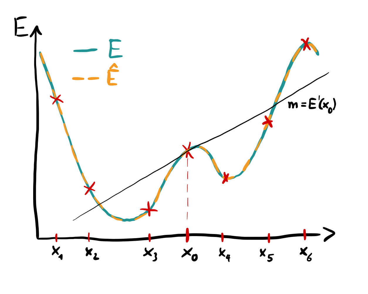
Function reconstruction and differentiation via parameter shifts.

Note

Before going through this tutorial, we recommend that readers refer to the Fourier series expressiveness tutorial. Additionally, having a basic understanding of the parameter-shift rule might make this tutorial easier to dive into.

Cost functions arising from quantum gates

We start our investigation by considering a cost function that arises from measuring the expectation value of an observable in a quantum state, created with a parametrized quantum operation that depends on a single variational parameter \(x\). That is, the state may be prepared by any circuit, but we will only allow a single parameter in a single operation to enter the circuit. For this we will use a handy gate structure that allows us to tune the complexity of the operation — and thus of the cost function. More concretely, we initialize a qubit register in a random state \(|\psi\rangle\) and apply a layer of Pauli-\(Z\) rotations RZ to all qubits, where all rotations are parametrized by the same angle \(x\). We then measure the expectation value of a random Hermitian observable \(B\) in the created state, so that our cost function overall has the form

\[E(x)=\langle\psi | U^\dagger(x) B U(x)|\psi\rangle.\]

Here, \(U(x)\) consists of a layer of RZ gates,

\[U(x)=\prod_{a=1}^N R_Z^{(a)}(x) = \prod_{a=1}^N \exp\left(-i\frac{x}{2} Z_a\right).\]

Let’s implement such a cost function using PennyLane. We begin with functions that generate the random initial state \(|\psi\rangle\) and the random observable \(B\) for a given number of qubits \(N\) and a fixed seed:

from scipy.stats import unitary_group
import numpy.random as rnd


def random_state(N, seed):
    """Create a random state on N qubits."""
    states = unitary_group.rvs(2 ** N, random_state=rnd.default_rng(seed))
    return states[0]


def random_observable(N, seed):
    """Create a random observable on N qubits."""
    rnd.seed(seed)
    # Generate real and imaginary part separately and (anti-)symmetrize them for Hermiticity
    real_part, imag_part = rnd.random((2, 2 ** N, 2 ** N))
    real_part += real_part.T
    imag_part -= imag_part.T
    return real_part + 1j * imag_part

Now let’s set up a “cost function generator”, namely a function that will create the cost function we discussed above, using \(|\psi\rangle\) as initial state and measuring the expectation value of \(B\). This generator has the advantage that we can quickly create the cost function for various numbers of qubits — and therefore cost functions with different complexity.

We will use the default qubit simulator with its JAX backend and also will rely on the NumPy implementation of JAX. To obtain precise results, we enable 64-bit float precision via the JAX config.

from jax.config import config

config.update("jax_enable_x64", True)
import jax
from jax import numpy as np
import pennylane as qml

def make_cost(N, seed):
    """Create a cost function on N qubits with N frequencies."""
    dev = qml.device("default.qubit", wires=N)

    @jax.jit
    @qml.qnode(dev, interface="jax")
    def cost(x):
        """Cost function on N qubits with N frequencies."""
        qml.QubitStateVector(random_state(N, seed), wires=dev.wires)
        for w in dev.wires:
            qml.RZ(x, wires=w, id="x")
        return qml.expval(qml.Hermitian(random_observable(N, seed), wires=dev.wires))

    return cost

We also prepare some plotting functionalities and colors:

import matplotlib.pyplot as plt

# Set a plotting range on the x-axis
xlim = (-np.pi, np.pi)
X = np.linspace(*xlim, 60)
# Colors
green = "#209494"
orange = "#ED7D31"
red = "xkcd:brick red"
blue = "xkcd:cerulean"
pink = "xkcd:bright pink"

Out:

No GPU/TPU found, falling back to CPU. (Set TF_CPP_MIN_LOG_LEVEL=0 and rerun for more info.)

Now that we took care of these preparations, let’s dive right into it: It can be shown 1 that \(E(x)\) takes the form of a Fourier series in the variable \(x\). That is to say that

\[E(x) = a_0 + \sum_{\ell=1}^R a_{\ell}\cos(\ell x)+b_{\ell}\sin(\ell x).\]

Here, \(a_{\ell}\) and \(b_{\ell}\) are the Fourier coefficients. If you would like to understand this a bit better still, have a read of fourier and remember to check out the Fourier module tutorial.

Due to \(B\) being Hermitian, \(E(x)\) is a real-valued function, so only positive frequencies and real coefficients appear in the Fourier series for \(E(x)\). This is true for any number of qubits (and therefore RZ gates) we use.

Using our function make_cost from above, we create the cost function for several numbers of qubits and store both the function and its evaluations on the plotting range X.

# Qubit numbers
Ns = [1, 2, 4, 5]
# Fix a seed
seed = 7658741

cost_functions = []
evaluated_cost = []
for N in Ns:
    # Generate the cost function for N qubits and evaluate it
    cost = make_cost(N, seed)
    evaluated_cost.append([cost(x) for x in X])
    cost_functions.append(cost)

Let’s take a look at the created \(E(x)\) for the various numbers of qubits:

# Figure with multiple axes
fig, axs = plt.subplots(1, len(Ns), figsize=(12, 2))

for ax, N, E in zip(axs, Ns, evaluated_cost):
    # Plot cost function evaluations
    ax.plot(X, E, color=green)
    # Axis and plot labels
    ax.set_title(f"{N} qubits")
    ax.set_xlabel("$x$")

_ = axs[0].set_ylabel("$E$")
plt.show()

Indeed we see that \(E(x)\) is a periodic function whose complexity grows when increasing \(N\) together with the number of RZ gates. To take a look at the frequencies that are present in these functions, we may use PennyLane’s fourier module.

Note

The analysis tool qnode_spectrum() makes use of the internal structure of the QNode that encodes the cost function. As we used the jax.jit decorator when defining the cost function above, we here need to pass the wrapped function to qnode_spectrum, which is stored in cost_function.__wrapped__.

from pennylane.fourier import qnode_spectrum

spectra = []
for N, cost_function in zip(Ns, cost_functions):
    # Compute spectrum with respect to parameter x
    spec = qnode_spectrum(cost_function.__wrapped__)(X[0])["x"][()]
    print(f"For {N} qubits the spectrum is {spec}.")
    # Store spectrum
    spectra.append([freq for freq in spec if freq>0.0])

Out:

For 1 qubits the spectrum is [-1.0, 0.0, 1.0].
For 2 qubits the spectrum is [-2.0, -1.0, 0.0, 1.0, 2.0].
For 4 qubits the spectrum is [-4.0, -3.0, -2.0, -1.0, 0.0, 1.0, 2.0, 3.0, 4.0].
For 5 qubits the spectrum is [-5.0, -4.0, -3.0, -2.0, -1.0, 0.0, 1.0, 2.0, 3.0, 4.0, 5.0].

The number of positive frequencies that appear in \(E(x)\) is the same as the number of RZ gates we used in the circuit! Recall that we only need to consider the positive frequencies because \(E(x)\) is real-valued, and that we accounted for the zero-frequency contribution in the coefficient \(a_0\). If you are interested why the number of gates coincides with the number of frequencies, check out the Fourier module tutorial.

Before moving on, let’s also have a look at the Fourier coefficients in the functions we created:

from pennylane.fourier.visualize import bar

fig, axs = plt.subplots(2, len(Ns), figsize=(12, 4.5))
for i, (cost_function, spec) in enumerate(zip(cost_functions, spectra)):
    # Compute the Fourier coefficients
    coeffs = qml.fourier.coefficients(cost_function, 1, len(spec)+2)
    # Show the Fourier coefficients
    bar(coeffs, 1, axs[:, i], show_freqs=True, colour_dict={"real": green, "imag": orange})
    axs[0, i].set_title(f"{Ns[i]} qubits")
    # Set x-axis labels
    axs[1, i].text(Ns[i] + 2, axs[1, i].get_ylim()[0], f"Frequency", ha="center", va="top")
    # Clean up y-axis labels
    if i == 0:
        _ = [axs[j, i].set_ylabel(lab) for j, lab in enumerate(["$a_\ell/2$", "$b_\ell/2$"])]
    else:
        _ = [axs[j, i].set_ylabel("") for j in [0, 1]]
plt.show()

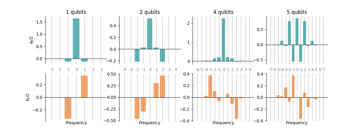
We find the real (imaginary) Fourier coefficients to be (anti-)symmetric. This is expected because \(E(x)\) is real-valued and we again see why it is enough to consider positive frequencies: the coefficients of the negative frequencies follow from those of the positive frequencies.

Determining the full dependence on \(x\)

Next we will show how to determine the full dependence of the cost function on \(x\), i.e., we will reconstruct \(E(x)\). The key idea is not new: Since \(E(x)\) is periodic with known, integer frequencies, we can reconstruct it exactly by using trigonometric interpolation. For this, we evaluate \(E\) at shifted positions \(x_\mu\). We will show the reconstruction both for equidistant and random shifts, corresponding to a uniform and a non-uniform discrete Fourier transform (DFT), respectively.

Equidistant shifts

For the equidistant case we can directly implement the trigonometric interpolation:

\[\begin{split}x_\mu &= \frac{2\mu\pi}{2R+1}\\ E(x) &=\sum_{\mu=-R}^R E\left(x_\mu\right) \frac{\sin\left(\frac{2R+1}{2}(x-x_\mu)\right)} {(2R+1)\sin \left(\frac{1}{2} (x-x_\mu)\right)},\\\end{split}\]

where we reformulated \(E\) in the second expression using the sinc function to enhance the numerical stability. Note that we have to take care of a rescaling factor of \(\pi\) between this definition of \(\operatorname{sinc}\) and the NumPy implementation np.sinc.

Note

When implementing \(E\), we will replace

\[\frac{\sin\left(\frac{2R+1}{2}(x-x_\mu)\right)} {(2R+1)\sin \left(\frac{1}{2} (x-x_\mu)\right)}\]

by

\[\frac{\operatorname{sinc}\left(\frac{2R+1}{2}(x-x_\mu)\right)} {\operatorname{sinc} \left(\frac{1}{2} (x-x_\mu)\right)}\]

where the sinc function is defined as \(\operatorname{sinc}(x)=\sin(x)/x\). This enhances the numerical stability since \(\operatorname{sinc}(0)=1\), so that the denominator does no longer vanish at the shifted points. Note that we have to take care of a rescaling factor of \(\pi\) between this definition of \(\operatorname{sinc}\) and the NumPy implementation np.sinc.

sinc = lambda x: np.sinc(x / np.pi)

def full_reconstruction_equ(fun, R):
    """Reconstruct a univariate function with up to R frequencies using equidistant shifts."""
    # Shift angles for the reconstruction
    shifts = [2 * mu * np.pi / (2 * R + 1) for mu in range(-R, R + 1)]
    # Shifted function evaluations
    evals = np.array([fun(shift) for shift in shifts])

    @jax.jit
    def reconstruction(x):
        """Univariate reconstruction using equidistant shifts."""
        kernels = np.array(
            [sinc((R + 0.5) * (x - shift)) / sinc(0.5 * (x - shift)) for shift in shifts]
        )
        return np.dot(evals, kernels)

    return reconstruction

reconstructions_equ = list(map(full_reconstruction_equ, cost_functions, Ns))

So how is this reconstruction doing? We will plot it along with the original function \(E\), mark the shifted evaluation points \(x_\mu\) (with crosses), and also show its deviation from \(E(x)\) (lower plots). For this, a function for the whole procedure of comparing the functions comes in handy, and we will reuse it further below. For convenience, showing the deviation will be an optional feature controled by the show_diff keyword argument.

def compare_functions(originals, reconstructions, Ns, shifts, show_diff=True):
    """Plot two sets of functions next to each other and show their difference (in pairs)."""
    # Prepare the axes; we need fewer axes if we don't show the deviations
    if show_diff:
        fig, axs = plt.subplots(2, len(originals), figsize=(12, 4.5))
    else:
        fig, axs = plt.subplots(1, len(originals), figsize=(12, 2))
    _axs = axs[0] if show_diff else axs

    # Run over the functions and reconstructions
    for i, (orig, recon, N, _shifts) in enumerate(zip(originals, reconstructions, Ns, shifts)):
        # Evaluate the original function and its reconstruction over the plotting range
        E = np.array(list(map(orig, X)))
        E_rec = np.array(list(map(recon, X)))
        # Evaluate the original function at the positions used in the reconstruction
        E_shifts = np.array(list(map(orig, _shifts)))

        # Show E, the reconstruction, and the shifts (top axes)
        _axs[i].plot(X, E, lw=2, color=orange)
        _axs[i].plot(X, E_rec, linestyle=":", lw=3, color=green)
        _axs[i].plot(_shifts, E_shifts, ls="", marker="x", c=red)
        # Manage plot titles and xticks
        _axs[i].set_title(f"{N} qubits")

        if show_diff:
            # [Optional] Show the reconstruction deviation (bottom axes)
            axs[1, i].plot(X, E - E_rec, color=blue)
            axs[1, i].set_xlabel("$x$")
            # Hide the xticks of the top x-axes if we use the bottom axes
            _axs[i].set_xticks([])

    # Manage y-axis labels
    _ = _axs[0].set_ylabel("$E$")
    if show_diff:
        _ = axs[1, 0].set_ylabel("$E-E_{rec}$")

    return fig, axs

equ_shifts = [[2 * mu * np.pi / (2 * N + 1) for mu in range(-N, N + 1)] for N in Ns]
fig, axs = compare_functions(cost_functions, reconstructions_equ, Ns, equ_shifts)
plt.show()

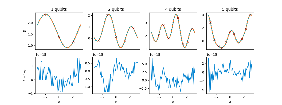
It works!

Non-equidistant shifts

Now let’s test the reconstruction with less regular sampling points on which to evaluate \(E\). This means we can no longer use the closed-form expression from above, but switch to solving the set of equations

\[E(x_\mu) = a_0 + \sum_{\ell=1}^R a_{\ell}\cos(\ell x_\mu)+b_{\ell}\sin(\ell x_\mu)\]

with the—now irregular—sampling points \(x_\mu\). For this, we set up the matrix

\[\begin{split}C_{\mu\ell} = \begin{cases} 1 &\text{ if } \ell=0\\ \cos(\ell x_\mu) &\text{ if } 1\leq\ell\leq R\\ \sin(\ell x_\mu) &\text{ if } R<\ell\leq 2R, \end{cases}\end{split}\]

collect the Fourier coefficients of \(E\) into the vector \(\boldsymbol{W}=(a_0, \boldsymbol{a}, \boldsymbol{b})\), and the evaluations of \(E\) into another vector called \(\boldsymbol{E}\) so that

\[\boldsymbol{E} = C \boldsymbol{W} \Rightarrow \boldsymbol{W} = C^{-1}\boldsymbol{E}.\]

Let’s implement this right away! We will take the function and the shifts \(x_\mu\) as inputs, inferring \(R\) from the number of the provided shifts, which is \(2R+1\).

def full_reconstruction_gen(fun, shifts):
    """Reconstruct a univariate trigonometric function using arbitrary shifts."""
    R = (len(shifts) - 1) // 2
    frequencies = np.array(list(range(1, R + 1)))

    # Construct the matrix C case by case
    C1 = np.ones((2 * R + 1, 1))
    C2 = np.cos(np.outer(shifts, frequencies))
    C3 = np.sin(np.outer(shifts, frequencies))
    C = np.hstack([C1, C2, C3])

    # Evaluate the function to reconstruct at the shifted positions
    evals = np.array(list(map(fun, shifts)))

    # Solve the system of linear equations by inverting C
    W = np.linalg.inv(C) @ evals

    # Extract the Fourier coefficients
    a0 = W[0]
    a = W[1 : R + 1]
    b = W[R + 1 :]

    # Construct the Fourier series
    @jax.jit
    def reconstruction(x):
        """Univariate reconstruction based on arbitrary shifts."""
        return a0 + np.dot(a, np.cos(frequencies * x)) + np.dot(b, np.sin(frequencies * x))

    return reconstruction

To see this version of the reconstruction in action, we will sample the shifts \(x_\mu\) at random in \([-\pi,\pi)\):

shifts = [rnd.random(2 * N + 1) * 2 * np.pi - np.pi for N in Ns]
reconstructions_gen = list(map(full_reconstruction_gen, cost_functions, shifts))
fig, axs = compare_functions(cost_functions, reconstructions_gen, Ns, shifts)
plt.show()

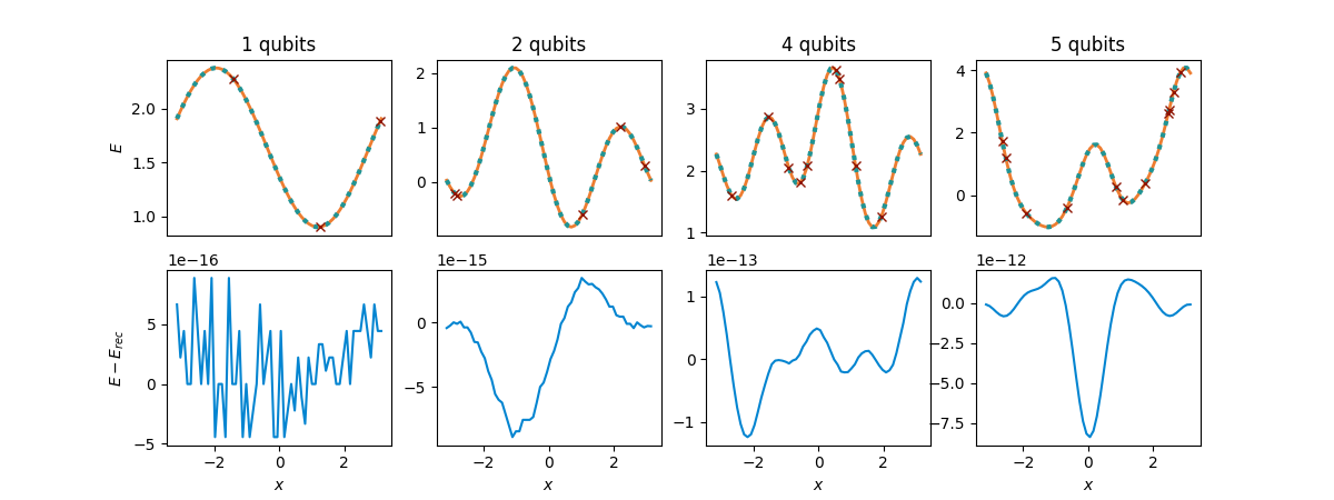
Again, we obtain a perfect reconstruction of \(E(x)\) up to numerical errors. We see that the deviation from the original cost function became larger than for equidistant shifts for some of the qubit numbers but it still remains much smaller than any energy scale of relevance in applications. The reason for these larger deviations is that some evaluation positions \(x_\mu\) were sampled very close to each other, so that inverting the matrix \(C\) becomes less stable numerically. Conceptually, we see that the reconstruction does not rely on equidistant evaluations points.

Note

For some applications, the number of frequencies \(R\) is not known exactly but an upper bound for \(R\) might be available. In this case, it is very useful that a reconstruction that assumes too many frequencies in \(E(x)\) works perfectly fine. However, it has the disadvantage of spending too many evaluations on the reconstruction, and the number of required measurements, which is meaningful for the (time) complexity of quantum algorithms, does so as well!

Differentiation via reconstructions

Next, we look at a modified reconstruction strategy that only obtains the odd or even part of \(E(x)\). This can be done by slightly modifying the shifted positions at which we evaluate \(E\) and the kernel functions.

From a perspective of implementing the derivatives there are two approaches, differing in which parts we derive on paper and which we leave to the computer: In the first approach, we perform a partial reconstruction using the evaluations of the original cost function \(E\) on the quantum computer, as detailed below. This gives us a function implemented in jax.numpy and we may afterwards apply jax.grad to this function and obtain the derivative function. \(E(0)\) then is only one evaluation of this function away. In the second approach, we compute the derivative of the partial reconstructions manually and directly implement the resulting shift rule that multiplies the quantum computer evaluations with coefficients and sums them up. This means that the partial reconstruction is not performed at all by the classical computer, but only was used on paper to derive the formula for the derivative.

Why do we look at both approaches?, you might ask. That is because neither of them is better than the other for all applications. The first approach offers us derivatives of any order without additional manual work by iteratively applying jax.grad, which is very convenient. However, the automatic differentiation via JAX becomes increasingly expensive with the order and we always reconstruct the same type of function, namely Fourier series, so that computing the respective derivatives once manually and coding up the resulting coefficients of the parameter-shift rule pays off in the long run. This is the strength of the second approach. We start with the first approach.

Automatically differentiated reconstructions

We implement the partial reconstruction method as a function; using PennyLane’s automatic differentiation backends, this then enables us to obtain the derivatives at the point of interest. For odd-order derivatives, we use the reconstruction of the odd part, for the even-order derivatives that of the even part.

We make use of modified Dirichlet kernels \(\tilde{D}_\mu(x)\) and equidistant shifts for this. For the odd reconstruction we have

\[\begin{split}E_\text{odd}(x) &= \sum_{\mu=1}^R E_\text{odd}(x_\mu) \tilde{D}_\mu(x)\\ \tilde{D}_\mu(x) &= \frac{\sin(R (x-x_\mu))}{2R \tan\left(\frac{1}{2} (x-x_\mu)\right)} - \frac{\sin(R (x+x_\mu))}{2R \tan\left(\frac{1}{2} (x+x_\mu)\right)},\end{split}\]

which we can implement using the reformulation

\[\frac{\sin(X)}{\tan(Y)}=\frac{X}{Y}\frac{\operatorname{sinc}(X)}{\operatorname{sinc}(Y)}\cos(Y)\]

for the kernel.

shifts_odd = lambda R: [(2 * mu - 1) * np.pi / (2 * R) for mu in range(1, R + 1)]
# Odd linear combination of Dirichlet kernels
D_odd = lambda x, R: np.array(
    [
        (
            sinc(R * (x - shift)) / sinc(0.5 * (x - shift)) * np.cos(0.5 * (x - shift))
            - sinc(R * (x + shift)) / sinc(0.5 * (x + shift)) * np.cos(0.5 * (x + shift))
        )
        for shift in shifts_odd(R)
    ]
)


def odd_reconstruction_equ(fun, R):
    """Reconstruct the odd part of an ``R``-frequency input function via equidistant shifts."""
    evaluations = np.array([(fun(shift) - fun(-shift)) / 2 for shift in shifts_odd(R)])

    @jax.jit
    def reconstruction(x):
        """Odd reconstruction based on equidistant shifts."""
        return np.dot(evaluations, D_odd(x, R))

    return reconstruction


odd_reconstructions = list(map(odd_reconstruction_equ, cost_functions, Ns))

The even part on the other hand takes the form

\[\begin{split}E_\text{even}(x) &= \sum_{\mu=0}^R E_\text{even}(x_\mu) \hat{D}_\mu(x)\\ \hat{D}_\mu(x) &= \begin{cases} \frac{\sin(Rx)}{2R \tan(x/2)} &\text{if } \mu = 0 \\[12pt] \frac{\sin(R (x-x_\mu))}{2R \tan\left(\frac{1}{2} (x-x_\mu)\right)} + \frac{\sin(R (x+x_\mu))}{2R \tan\left(\frac{1}{2} (x+x_\mu)\right)} & \text{if } \mu \in [R-1] \\[12pt] \frac{\sin(R (x-\pi))}{2R \tan\left(\frac{1}{2} (x-\pi)\right)} & \text{if } \mu = R. \end{cases}\end{split}\]

Note that not only the kernels \(\hat{D}_\mu(x)\) but also the shifted positions \(\{x_\mu\}\) differ between the odd and even case.

shifts_even = lambda R: [mu * np.pi / R for mu in range(1, R)]
# Even linear combination of Dirichlet kernels
D_even = lambda x, R: np.array(
    [
        (
            sinc(R * (x - shift)) / sinc(0.5 * (x - shift)) * np.cos(0.5 * (x - shift))
            + sinc(R * (x + shift)) / sinc(0.5 * (x + shift)) * np.cos(0.5 * (x + shift))
        )
        for shift in shifts_even(R)
    ]
)
# Special cases of even kernels
D0 = lambda x, R: sinc(R * x) / (sinc(x / 2)) * np.cos(x / 2)
Dpi = lambda x, R: sinc(R * (x - np.pi)) / sinc((x - np.pi) / 2) * np.cos((x - np.pi) / 2)


def even_reconstruction_equ(fun, R):
    """Reconstruct the even part of ``R``-frequency input function via equidistant shifts."""
    _evaluations = np.array([(fun(shift) + fun(-shift)) / 2 for shift in shifts_even(R)])
    evaluations = np.array([fun(0), *_evaluations, fun(np.pi)])
    kernels = lambda x: np.array([D0(x, R), *D_even(x, R), Dpi(x, R)])

    @jax.jit
    def reconstruction(x):
        """Even reconstruction based on equidistant shifts."""
        return np.dot(evaluations, kernels(x))

    return reconstruction


even_reconstructions = list(map(even_reconstruction_equ, cost_functions, Ns))

We also set up a function that performs both partial reconstructions and sums the resulting functions to the full Fourier series.

def summed_reconstruction_equ(fun, R):
    """Sum an odd and an even reconstruction into the full function."""
    _odd_part = odd_reconstruction_equ(fun, R)
    _even_part = even_reconstruction_equ(fun, R)

    def reconstruction(x):
        """Full function based on separate odd/even reconstructions."""
        return _odd_part(x) + _even_part(x)

    return reconstruction


summed_reconstructions = list(map(summed_reconstruction_equ, cost_functions, Ns))

We show these even (blue) and odd (red) reconstructions and how they indeed sum to the full function (orange, dashed). We will again use the compare_functions utility from above for the comparison.

from matplotlib.lines import Line2D

# Obtain the shifts for the reconstruction of both parts
odd_and_even_shifts = [
    (
        shifts_odd(R)
        + shifts_even(R)
        + list(-1 * np.array(shifts_odd(R)))
        + list(-1 * np.array(shifts_odd(R)))
        + [0, np.pi]
    )
    for R in Ns
]

# Show the reconstructed parts and the sums
fig, axs = compare_functions(cost_functions, summed_reconstructions, Ns, odd_and_even_shifts)
for i, (odd_recon, even_recon) in enumerate(zip(odd_reconstructions, even_reconstructions)):
    # Odd part
    E_odd = np.array(list(map(odd_recon, X)))
    axs[0, i].plot(X, E_odd, color=red)
    # Even part
    E_even = np.array(list(map(even_recon, X)))
    axs[0, i].plot(X, E_even, color=blue)
    axs[0, i].set_title('')
_ = axs[1, 0].set_ylabel("$E-(E_{odd}+E_{even})$")
colors = [green, red, blue, orange]
styles = ['-', '-', '-', '--']
handles = [Line2D([0], [0], color=c, ls=ls, lw=1.2) for c, ls in zip(colors, styles)]
labels = ['Original', 'Odd reconstruction', 'Even reconstruction', 'Summed reconstruction']
_ = fig.legend(handles, labels, bbox_to_anchor=(0.2, 0.89), loc='lower left', ncol=4)
plt.show()

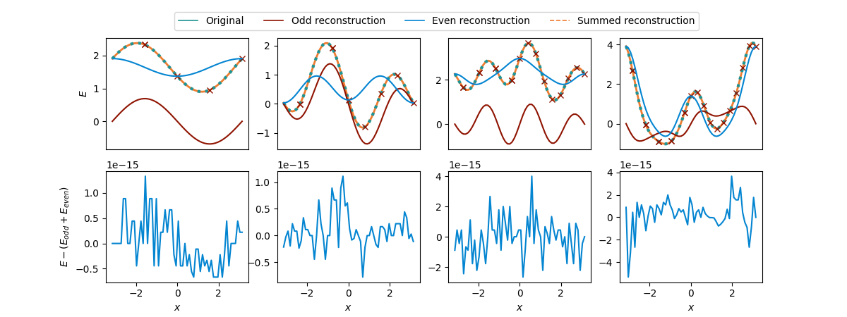
Great! The even and odd part indeed sum to the correct function again. But what did we gain?

Nothing, actually, for the full reconstruction! Quite the opposite, we spent \(2R\) evaluations of \(E\) on each part, that is \(4R\) evaluations overall to obtain a description of the full function \(E\)! This is way more than the \(2R+1\) evaluations needed for the full reconstructions from the beginning.

However, remember that we set out to compute derivatives of \(E\) at \(0\), so that for derivatives of odd/even order only the odd/even reconstruction is required. Using an autodifferentiation framework, e.g. JAX, we can easily compute such higher-order derivatives:

# An iterative function computing the ``order``th derivative of a function ``f`` with JAX
grad_gen = lambda f, order: grad_gen(jax.grad(f), order - 1) if order > 0 else f

# Compute the first, second, and fourth derivative
for order, name in zip([1, 2, 4], ["First", "Second", "4th"]):
    recons = odd_reconstructions if order % 2 else even_reconstructions
    recon_name = "odd " if order % 2 else "even"
    cost_grads = np.array([grad_gen(orig, order)(0.0) for orig in cost_functions])
    recon_grads = np.array([grad_gen(recon, order)(0.0) for recon in recons])
    all_equal = (
        "All entries match" if np.allclose(cost_grads, recon_grads) else "Some entries differ!"
    )
    print(f"{name} derivatives via jax: {all_equal}")
    print("From the cost functions:       ", np.round(np.array(cost_grads), 6))
    print(f"From the {recon_name} reconstructions: ", np.round(np.array(recon_grads), 6), "\n")

Out:

First derivatives via jax: All entries match
From the cost functions:        [-0.689767 -2.463189  2.704583  1.935272]
From the odd  reconstructions:  [-0.689767 -2.463189  2.704583  1.935272]

Second derivatives via jax: All entries match
From the cost functions:        [ 0.26814   1.696854 -2.055918 -7.236953]
From the even reconstructions:  [ 0.26814   1.696854 -2.055918 -7.236953]

4th derivatives via jax: All entries match
From the cost functions:        [-0.26814  -6.938376 15.640123 53.355635]
From the even reconstructions:  [-0.26814  -6.938376 15.640123 53.355635]

The derivatives coincide.

Note

While we used the \(2R+1\) evaluations \(x_\mu=\frac{2\mu\pi}{2R+1}\) for the full reconstruction, derivatives only require \(2R\) calls to the respective circuit. Also note that the derivatives can be computed at any position \(x_0\) other than \(0\) by simply reconstructing the function \(E(x+x_0)\), which again will be a Fourier series like \(E(x)\).

Generalized parameter-shift rules

The second method is based on the previous one. Instead of consulting JAX, we may compute the wanted derivative of the odd/even kernel function manually and thus derive general parameter-shift rules from this. We will leave the technical derivation of these rules to the paper 1. Start with the first derivative, which certainly is used the most:

\[E'(0) = \sum_{\mu=1}^{2R} E\left(\frac{2\mu-1}{2R}\pi\right) \frac{(-1)^{\mu-1}}{4R\sin^2\left(\frac{2\mu-1}{4R}\pi\right)},\]

This is straight-forward to implement by defining the coefficients and evaluating \(E\) at the shifted positions \(x_\mu\):

def parameter_shift_first(fun, R):
    """Compute the first-order derivative of a function with R frequencies at 0."""
    shifts = (2 * np.arange(1, 2 * R + 1) - 1) * np.pi / (4 * R)
    # Classically computed coefficients
    coeffs = np.array(
        [(-1) ** mu / (4 * R * np.sin(shift) ** 2) for mu, shift in enumerate(shifts)]
    )
    # Evaluations of the cost function E(x_mu)
    evaluations = np.array(list(map(fun, 2 * shifts)))
    # Contract coefficients with evaluations
    return np.dot(coeffs, evaluations)

ps_der1 = list(map(parameter_shift_first, cost_functions, Ns))

The second-order derivative takes a similar form, but we have to take care of the evaluation at \(0\) and the corresponding coefficient separately:

\[E''(0) = -E(0)\frac{2R^2+1}{6} - \sum_{\mu=1}^{2R-1} E\left(\frac{\mu\pi}{R}\right)\frac{(-1)^\mu}{2\sin^2 \left(\frac{\mu\pi}{2R}\right)}.\]

Let’s code this up, again we only get slight complications from the special evaluation at \(0\):

def parameter_shift_second(fun, R):
    """Compute the second-order derivative of a function with R frequencies at 0."""
    shifts = np.arange(1, 2 * R) * np.pi / (2 * R)
    # Classically computed coefficients for the main sum
    _coeffs = [(-1) ** mu / (2 * np.sin(shift) ** 2) for mu, shift in enumerate(shifts)]
    # Include the coefficients for the "special" term E(0).
    coeffs = np.array([-(2 * R ** 2 + 1) / 6] + _coeffs)
    # Evaluate at the regularily shifted positions
    _evaluations = list(map(fun, 2 * shifts))
    # Include the "special" term E(0).
    evaluations = np.array([fun(0.0)] + _evaluations)
    # Contract coefficients with evaluations.
    return np.dot(coeffs, evaluations)

ps_der2 = list(map(parameter_shift_second, cost_functions, Ns))

We will compare these two shift rules to the finite-difference derivative commonly used for numerical differentiation. We choose a finite difference of \(d_x=5\times 10^{-5}\).

dx = 5e-5

def finite_diff_first(fun):
    """Compute the first order finite difference derivative."""
    return (fun(dx/2) - fun(-dx/2))/dx

fd_der1 = list(map(finite_diff_first, cost_functions))

def finite_diff_second(fun):
    """Compute the second order finite difference derivative."""
    fun_p, fun_0, fun_m = fun(dx), fun(0.0), fun(-dx)
    return ((fun_p - fun_0)/dx - (fun_0 - fun_m)/dx) /dx

fd_der2 = list(map(finite_diff_second, cost_functions))

All that is left is to compare the computed parameter-shift and finite-difference derivatives:

print("Number of qubits/RZ gates:         ", *Ns, sep=" " * 9)
print(f"First-order parameter-shift rule:  {np.round(np.array(ps_der1), 6)}")
print(f"First-order finite difference:     {np.round(np.array(fd_der1), 6)}")
print(f"Second-order parameter-shift rule: {np.round(np.array(ps_der2), 6)}")
print(f"Second-order finite difference:    {np.round(np.array(fd_der2), 6)}")

Out:

Number of qubits/RZ gates:                  1         2         4         5
First-order parameter-shift rule:  [-0.689767 -2.463189  2.704583  1.935272]
First-order finite difference:     [-0.689767 -2.463189  2.704583  1.935272]
Second-order parameter-shift rule: [ 0.26814   1.696854 -2.055918 -7.236953]
Second-order finite difference:    [ 0.268141  1.696854 -2.055919 -7.236953]

The parameter-shift rules work as expected! And we were able to save a circuit evaluation as compared to a full reconstruction.

And this is all we want to show here about univariate function reconstructions and generalized parameter shift rules. Note that the techniques above can partially be extended to frequencies that are not integer-valued, but many closed form expressions are no longer valid. For the reconstruction, the approach via Dirichlet kernels no longer works in the general case; instead, a system of equations has to be solved, but with generalized frequencies \(\{\Omega_\ell\}\) instead of \(\{\ell\}\) (see e.g. Sections III A-C in 1)

References

1(1,2,3,4,5)

David Wierichs, Josh Izaac, Cody Wang, Cedric Yen-Yu Lin. “General parameter-shift rules for quantum gradients”. arXiv preprint arXiv:2107.12390.

2

Javier Gil Vidal, Dirk Oliver Theis. “Calculus on parameterized quantum circuits”. arXiv preprint arXiv:1812.06323.

3

Mateusz Ostaszewski, Edward Grant, Marcello Benedetti. “Structure optimization for parameterized quantum circuits”. arXiv preprint arXiv:1905.09692.

4

Artur F. Izmaylov, Robert A. Lang, Tzu-Ching Yen. “Analytic gradients in variational quantum algorithms: Algebraic extensions of the parameter-shift rule to general unitary transformations”. arXiv preprint arXiv:2107.08131.

5

Oleksandr Kyriienko, Vincent E. Elfving. “Generalized quantum circuit differentiation rules”. arXiv preprint arXiv:2108.01218.

About the author

David Wierichs

David is a researcher and quantum software developer at Xanadu, who likes to think about quantum gradients and how to use them in variational quantum algorithms. He enjoys sharing ideas in science and open source software and likes implementing cool stuff in PennyLane.

demos/tutorial_general_parshift

 

Download Python script

 

Download Notebook

 

View on GitHub