Feedback-Based Quantum Optimization (FALQON)

Authors: David Wakeham and Jack Ceroni — Posted: 21 May 2021. Last updated: 21 May 2021.

---

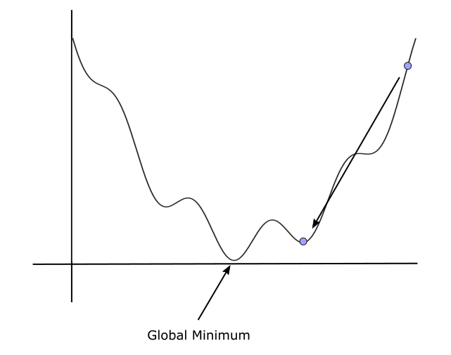
While the Quantum Approximate Optimization Algorithm (QAOA) is one of the best-known processes for solving combinatorial optimization problems with quantum computers, it has a major drawback: convergence isn’t guaranteed, as the optimization procedure can become “stuck” in local minima.

This tutorial explores the FALQON algorithm introduced in a recent paper by Magann et al. It is similar in spirit to QAOA, but uses iterative feedback steps rather than a global optimization over parameters, avoiding the use of a classical optimizer.

In this demo, we will implement FALQON to solve the MaxClique problem in graph theory, perform benchmarking, and combine FALQON with QAOA to create a powerful optimization procedure.

Note

If you are not familiar with QAOA, we recommend checking out the Intro to QAOA tutorial, since many of the same ideas carry over and will be used throughout this demonstration.

Theory

To solve a combinatorial optimization problem with a quantum computer, a typical strategy is to encode the solution to the problem as the ground state of a cost Hamiltonian \(H_c\). Then, we use some procedure to drive an initial state into the ground state of \(H_c\). FALQON falls under this broad scheme.

Consider a quantum system governed by a Hamiltonian of the form \(H = H_c + \beta(t) H_d\). These kinds of Hamiltonians appear often in the theory of quantum control, a field of inquiry which studies how a quantum system can be driven from one state to another. The choice of \(\beta(t)\) corresponds to a “driving strategy”, which partially determines how the system evolves with time.

Suppose our objective is to drive some quantum system to the ground state of \(H_c\). It is a reasonable goal to construct a quantum control process such that the energy expectation \(\langle H_c \rangle_t\) decreases with time:

\[\frac{d}{dt} \langle H_c\rangle_t = \frac{d}{dt} \langle \psi(t)|H_c|\psi(t)\rangle = i \beta(t)\langle [H_d, H_c] \rangle_t \leq 0,\]

where the product rule and the Schrödinger equation are used to derive the above formula. If we pick \(\beta(t) = -\langle i[H_d, H_c] \rangle_t,\) so that

\[\frac{d}{dt} \langle H_c\rangle_t = -|\langle i[H_d, H_c] \rangle_t|^2 \leq 0,\]

then \(\langle H_c \rangle\) is guaranteed to strictly decrease, as desired! Thus, if we evolve some initial state \(|\psi_0\rangle\) under the time evolution operator \(U\) corresponding to \(H\),

\[U(T) = \mathcal{T} \exp \Big[ -i \displaystyle\int_{0}^{T} H(t) \ dt \Big] \approx \mathcal{T} \exp \Big[ -i \displaystyle\sum_{k = 0}^{T/\Delta t} H( k \Delta t) \Delta t \Big],\]

where \(\mathcal{T}\) is the time-ordering operator and \(\Delta t\) is some small time step, then the energy expectation will strictly decrease, for a large enough value of \(T\). This is exactly the procedure used by FALQON to minimize \(\langle H_c \rangle\). In general, implementing a time evolution unitary in a quantum circuit is difficult, so we use a Trotter-Suzuki decomposition to perform approximate time evolution. We then have

\[U(T) \approx \mathcal{T} \exp \Big[ -i \displaystyle\sum_{k = 0}^{T/\Delta t} H( k \Delta t) \Delta t \Big] \approx e^{-i\beta_n H_d \Delta t} e^{-iH_c \Delta t} \cdots e^{-i\beta_1 H_d \Delta t} e^{-iH_c \Delta t} = U_d(\beta_n) U_c \cdots U_d(\beta_1) U_c,\]

where \(n = T/\Delta t\) and \(\beta_k = \beta(k\Delta t)\). For each layer of the time evolution, the value \(\beta_k\) is required. However, \(\beta_k\) is dependent on the state of the system at some time. Recall that

\[\beta(t) = - \langle \psi(t) | i [H_d, H_c] | \psi(t) \rangle.\]

We let \(A(t) := i\langle [H_d, H_c] \rangle_t\). Our strategy is to obtain the values \(\beta_k\) recursively, by finding the value of \(A(t)\) for the previous time step. We then set

\[\beta_{k+1} = -A_k = -A(k\Delta t).\]

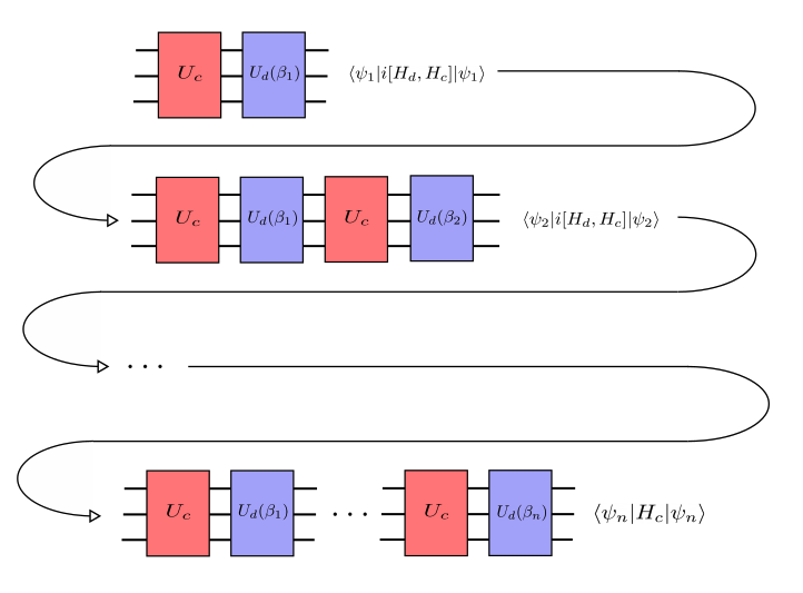
This leads to the FALQON algorithm as a recursive process. On step \(k\), we perform the following three substeps:

1. Prepare the state \(|\psi_k\rangle = U_d(\beta_k) U_c \cdots U_d(\beta_1) U_c|\psi_0\rangle\).

2. Measure the expectation value \(A_k = \langle i[H_c, H_d]\rangle_{k \Delta t}\).

3. Set \(\beta_{k+1} = -A_k\).

We repeat for all \(k\) from \(1\) to \(n\), where \(n\) is a hyperparameter. At the final step we evaluate \(\langle H_c \rangle\), which gives us an approximation for the ground state of \(H_c\).

Simulating FALQON with PennyLane

To begin, we import the necessary dependencies:

import pennylane as qml
from pennylane import numpy as np
from matplotlib import pyplot as plt
from pennylane import qaoa as qaoa
import networkx as nx

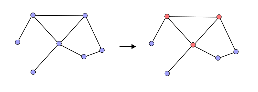
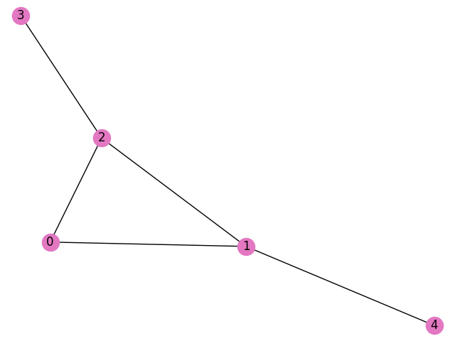
In this demonstration, we will be using FALQON to solve the maximum clique (MaxClique) problem: finding the largest complete subgraph of some graph \(G\). For example, the following graph’s maximum clique is coloured in red:

We attempt to find the maximum clique of the graph below:

edges = [(0, 1), (1, 2), (2, 0), (2, 3), (1, 4)]
graph = nx.Graph(edges)
nx.draw(graph, with_labels=True, node_color="#e377c2")

We must first encode this combinatorial problem into a cost Hamiltonian \(H_c\). This ends up being

\[H_c = 3 \sum_{(i, j) \in E(\bar{G})} (Z_i Z_j - Z_i - Z_j) + \displaystyle\sum_{i \in V(G)} Z_i,\]

where each qubit is a node in the graph, and the states \(|0\rangle\) and \(|1\rangle\) represent whether the vertex has been marked as part of the clique, as is the case for most standard QAOA encoding schemes. Note that \(\bar{G}\) is the complement of \(G\): the graph formed by connecting all nodes that do not share an edge in \(G\).

In addition to defining \(H_c\), we also require a driver Hamiltonian \(H_d\) which does not commute with \(H_c\). The driver Hamiltonian’s role is similar to that of the mixer Hamiltonian in QAOA. To keep things simple, we choose a sum over Pauli \(X\) operations on each qubit:

\[H_d = \displaystyle\sum_{i \in V(G)} X_i.\]

These Hamiltonians come nicely bundled together in the PennyLane QAOA module:

cost_h, driver_h = qaoa.max_clique(graph, constrained=False)

print("Cost Hamiltonian")
print(cost_h)
print("Driver Hamiltonian")
print(driver_h)

Out:

Cost Hamiltonian
  (-1.25) [Z3]
+ (-1.25) [Z4]
+ (-0.5) [Z0]
+ (0.25) [Z1]
+ (0.25) [Z2]
+ (0.75) [Z0 Z3]
+ (0.75) [Z0 Z4]
+ (0.75) [Z1 Z3]
+ (0.75) [Z2 Z4]
+ (0.75) [Z3 Z4]
Driver Hamiltonian
  (1) [X0]
+ (1) [X1]
+ (1) [X2]
+ (1) [X3]
+ (1) [X4]

One of the main ingredients in the FALQON algorithm is the operator \(i [H_d, H_c]\). In the case of MaxClique, we can write down the commutator \([H_d, H_c]\) explicitly:

\[[H_d, H_c] = 3 \displaystyle\sum_{k \in V(G)} \displaystyle\sum_{(i, j) \in E(\bar{G})} \big( [X_k, Z_i Z_j] - [X_k, Z_i] - [X_k, Z_j] \big) + 3 \displaystyle\sum_{i \in V(G)} \displaystyle\sum_{j \in V(G)} [X_i, Z_j].\]

There are two distinct commutators that we must calculate, \([X_k, Z_j]\) and \([X_k, Z_i Z_j]\). This is straightforward as we know exactly what the commutators of the Pauli matrices are. We have:

\[[X_k, Z_j] = -2 i \delta_{kj} Y_k \ \ \ \text{and} \ \ \ [X_k, Z_i Z_j] = -2 i \delta_{ik} Y_k Z_j - 2i \delta_{jk} Z_i Y_k,\]

where \(\delta_{kj}\) is the Kronecker delta. Therefore it follows from substitution into the above equation and multiplication by \(i\) that:

\[i [H_d, H_c] = 6 \displaystyle\sum_{k \in V(G)} \displaystyle\sum_{(i, j) \in E(\bar{G})} \big( \delta_{ki} Y_k Z_j + \delta_{kj} Z_{i} Y_{k} - \delta_{ki} Y_k - \delta_{kj} Y_k \big) + 6 \displaystyle\sum_{i \in V(G)} Y_{i}.\]

This new operator has quite a few terms! Therefore, we write a short method which computes it for us, and returns a Hamiltonian object. Note that this method works for any graph:

def build_hamiltonian(graph):
    H = qml.Hamiltonian([], [])

    # Computes the complement of the graph
    graph_c = nx.complement(graph)

    for k in graph_c.nodes:
        # Adds the terms in the first sum
        for edge in graph_c.edges:
            i, j = edge
            if k == i:
                H += 6 * (qml.PauliY(k) @ qml.PauliZ(j) - qml.PauliY(k))
            if k == j:
                H += 6 * (qml.PauliZ(i) @ qml.PauliY(k) - qml.PauliY(k))
        # Adds the terms in the second sum
        H += 6 * qml.PauliY(k)

    return H


print("MaxClique Commutator")
print(build_hamiltonian(graph))

Out:

MaxClique Commutator
  (-12.0) [Y3]
+ (-12.0) [Y4]
+ (-6.0) [Y0]
+ (6.0) [Y0 Z3]
+ (6.0) [Y0 Z4]
+ (6.0) [Y1 Z3]
+ (6.0) [Y2 Z4]
+ (6.0) [Z0 Y3]
+ (6.0) [Z1 Y3]
+ (6.0) [Y3 Z4]
+ (6.0) [Z0 Y4]
+ (6.0) [Z2 Y4]
+ (6.0) [Z3 Y4]

We can now build the FALQON algorithm. Our goal is to evolve some initial state under the Hamiltonian \(H\), with our chosen \(\beta(t)\). We first define one layer of the Trotterized time evolution, which is of the form \(U_d(\beta_k) U_c\). Note that we can use the ApproxTimeEvolution template:

def falqon_layer(beta_k, cost_h, driver_h, delta_t):
    qml.ApproxTimeEvolution(cost_h, delta_t, 1)
    qml.ApproxTimeEvolution(driver_h, delta_t * beta_k, 1)

We then define a method which returns a FALQON ansatz corresponding to a particular cost Hamiltonian, driver Hamiltonian, and \(\Delta t\). This involves multiple repetitions of the “FALQON layer” defined above. The initial state of our circuit is an even superposition:

def build_maxclique_ansatz(cost_h, driver_h, delta_t):
    def ansatz(beta, **kwargs):
        layers = len(beta)
        for w in dev.wires:
            qml.Hadamard(wires=w)
        qml.layer(
            falqon_layer,
            layers,
            beta,
            cost_h=cost_h,
            driver_h=driver_h,
            delta_t=delta_t
        )

    return ansatz


def expval_circuit(beta, measurement_h):
    ansatz = build_maxclique_ansatz(cost_h, driver_h, delta_t)
    ansatz(beta)
    return qml.expval(measurement_h)

Finally, we implement the recursive process, where FALQON is able to determine the values of \(\beta_k\), feeding back into itself as the number of layers increases. This is straightforward using the methods defined above:

def max_clique_falqon(graph, n, beta_1, delta_t, dev):
    comm_h = build_hamiltonian(graph) # Builds the commutator
    cost_h, driver_h = qaoa.max_clique(graph, constrained=False) # Builds H_c and H_d
    cost_fn = qml.QNode(expval_circuit, dev, interface="autograd") # The ansatz + measurement circuit is executable

    beta = [beta_1] # Records each value of beta_k
    energies = [] # Records the value of the cost function at each step

    for i in range(n):
        # Adds a value of beta to the list and evaluates the cost function
        beta.append(-1 * cost_fn(beta, measurement_h=comm_h))  # this call measures the expectation of the commuter hamiltonian
        energy = cost_fn(beta, measurement_h=cost_h)  # this call measures the expectation of the cost hamiltonian
        energies.append(energy)

    return beta, energies

Note that we return both the list of \(\beta_k\) values, as well as the expectation value of the cost Hamiltonian for each step.

We can now run FALQON for our MaxClique problem! It is important that we choose \(\Delta t\) small enough such that the approximate time evolution is close enough to the real time evolution, otherwise we the expectation value of \(H_c\) may not strictly decrease. For this demonstration, we set \(\Delta t = 0.03\), \(n = 40\), and \(\beta_1 = 0\). These are comparable to the hyperparameters chosen in the original paper.

n = 40
beta_1 = 0.0
delta_t = 0.03

dev = qml.device("default.qubit", wires=graph.nodes) # Creates a device for the simulation
res_beta, res_energies = max_clique_falqon(graph, n, beta_1, delta_t, dev)

We can then plot the expectation value of the cost Hamiltonian over the iterations of the algorithm:

plt.plot(range(n+1)[1:], res_energies)
plt.xlabel("Iteration")
plt.ylabel("Cost Function Value")
plt.show()

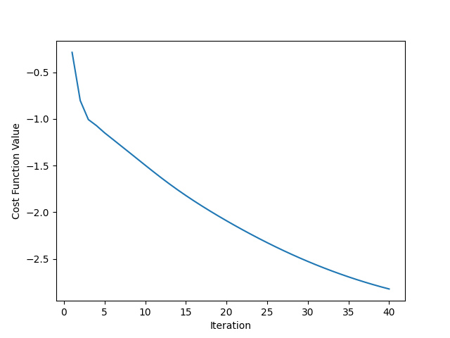
The expectation value decreases!

To get a better understanding of the performance of the FALQON algorithm, we can create a graph showing the probability of measuring each possible bit string. We define the following circuit, feeding in the optimal values of \(\beta_k\):

@qml.qnode(dev, interface="autograd")
def prob_circuit():
    ansatz = build_maxclique_ansatz(cost_h, driver_h, delta_t)
    ansatz(res_beta)
    return qml.probs(wires=dev.wires)

Running this circuit gives us the following probability distribution:

probs = prob_circuit()
plt.bar(range(2**len(dev.wires)), probs)
plt.xlabel("Bit string")
plt.ylabel("Measurement Probability")
plt.show()

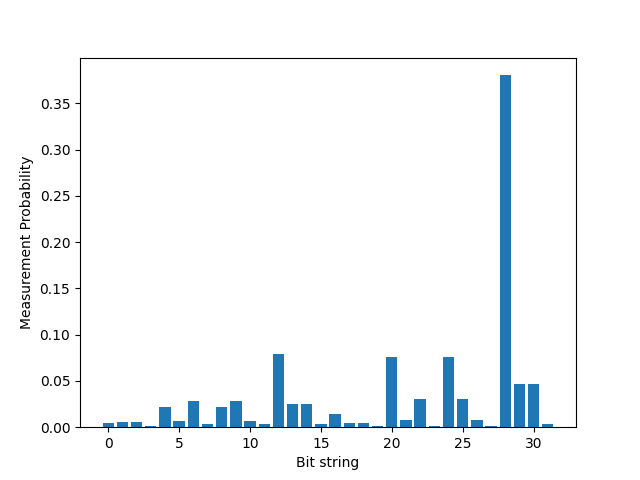
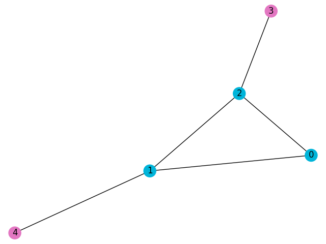
The bit string occurring with the highest probability is the state \(|28\rangle = |11100\rangle\). This corresponds to nodes \(0\), \(1\), and \(2\), which is precisely the maximum clique. FALQON has solved the MaxClique problem 🤩.

graph = nx.Graph(edges)
cmap = ["#00b4d9"]*3 + ["#e377c2"]*2
nx.draw(graph, with_labels=True, node_color=cmap)

Benchmarking FALQON

After seeing how FALQON works, it is worth considering how well FALQON performs according to a set of benchmarking criteria on a batch of graphs. We generate graphs randomly using the Erdos-Renyi model, where we start with the complete graph on \(n\) vertices and then keep each edge with probability \(p\). We then find the maximum cliques on these graphs using the Bron-Kerbosch algorithm. To benchmark FALQON, the relative error in the estimated minimum energy

\[r_A = \frac{\langle H_C\rangle - \langle H_C\rangle_\text{min}}{|\langle H_C\rangle_\text{min}|}\]

makes a good figure of merit.

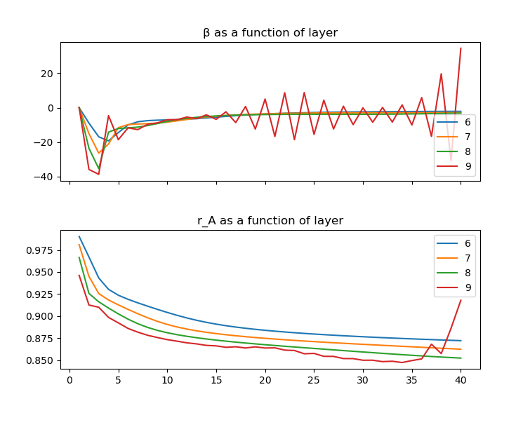
Final results for \(r_A\), along with \(\beta\), are plotted below, with the number of FALQON layers on the horizontal axis. We have averaged over \(50\) random graphs per node size, for sizes \(n = 6, 7, 8, 9\), with probability \(p = 0.1\) of keeping an edge. Running FALQON for \(40\) steps, with \(\Delta t = 0.01\), produces:

The relative error decreases with the number of layers (as we expect from the construction) and graph size (suggesting the errors grows more slowly than the minimum energy). The exception is \(n = 9\), where the step size has become too large and the Trotter-Suzuki decomposition breaks down. The rate of decrease also slows down. Even though the algorithm will converge to the ground state, it won’t always get there in a few time steps!

Seeding QAOA with FALQON (Bird Seed 🦅)

Both FALQON and QAOA have unique benefits and drawbacks. While FALQON requires no classical optimization and is guaranteed to decrease the cost function with each iteration, its circuit depth grows linearly with the number of iterations. The benchmarking data also shows how the reduction in cost slows with each layer, and the additional burden of correctly tuning the time step. On the other hand, QAOA has a fixed circuit depth, but does require classical optimization, and is therefore subject to all of the drawbacks that come with probing a cost landscape for a set of optimal parameters.

QAOA and FALQON also have many similarities, most notably, their circuit structure. Both involve alternating layers of time evolution operators corresponding to a cost and a mixer/driver Hamiltonian. The FALQON paper raises the idea of combining FALQON and QAOA to yield a new optimization algorithm that leverages the benefits of both. In this final section of the tutorial, we will implement this procedure in PennyLane.

Suppose we want to run a QAOA circuit of depth \(p\). Our ansatz will be of the form

\[U_{\text{QAOA}} = e^{-i \alpha_p H_m} e^{-i \gamma_p H_c} \cdots e^{-i \alpha_1 H_m} e^{-i \gamma_1 H_c},\]

for sets of parameters \(\{\alpha_k\}\) and \(\{\gamma_k\}\), which are optimized. If we run FALQON for \(p\) steps, setting \(H_d = H_m\), and use the same cost Hamiltonian, we will end up with the following ansatz:

\[U_{\text{FALQON}} = e^{-i \Delta t \beta_p H_m} e^{-i \Delta t H_c} \cdots e^{-i \Delta t \beta_1 H_m} e^{-i \Delta t H_c}.\]

Thus, our strategy is to initialize our QAOA parameters using the \(\beta_k\) values that FALQON yields. More specifically, we set \(\alpha_k = \Delta t \beta_k\) and \(\gamma_k = \Delta t\). We then optimize over these parameters. The goal is that these parameters provide QAOA a good place in the parameter space to begin its optimization.

Using the code from earlier in the demonstration, we can easily prototype this process. To illustrate the power of this new technique, we attempt to solve MaxClique on a slightly more complicated graph:

new_edges = [(0, 1), (1, 2), (2, 0), (2, 3), (1, 4), (4, 5), (5, 2), (0, 6)]
new_graph = nx.Graph(new_edges)
nx.draw(new_graph, with_labels=True, node_color="#e377c2")

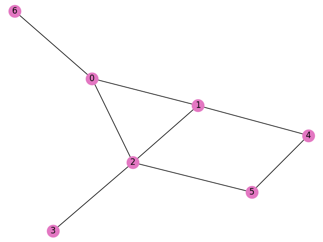
We can now use the PennyLane QAOA module to create a QAOA circuit corresponding to the MaxClique problem. For this demonstration, we set the depth to \(5\):

depth = 5
dev = qml.device("default.qubit", wires=new_graph.nodes)

# Creates the cost and mixer Hamiltonians
cost_h, mixer_h = qaoa.max_clique(new_graph, constrained=False)

# Creates a layer of QAOA
def qaoa_layer(gamma, beta):
    qaoa.cost_layer(gamma, cost_h)
    qaoa.mixer_layer(beta, mixer_h)

# Creates the full QAOA circuit as an executable cost function
def qaoa_circuit(params, **kwargs):
    for w in dev.wires:
        qml.Hadamard(wires=w)
    qml.layer(qaoa_layer, depth, params[0], params[1])


@qml.qnode(dev, interface="autograd")
def qaoa_expval(params):
    qaoa_circuit(params)
    return qml.expval(cost_h)

Now all we have to do is run FALQON for \(5\) steps to get our initial QAOA parameters. We set \(\Delta t = 0.02\):

delta_t = 0.02

res, res_energy = max_clique_falqon(new_graph, depth-1, 0.0, delta_t, dev)

params = np.array([[delta_t for k in res], [delta_t * k for k in res]], requires_grad=True)

Finally, we run our QAOA optimization procedure. We set the number of QAOA executions to \(40\):

steps = 40

optimizer = qml.GradientDescentOptimizer()

for s in range(steps):
    params, cost = optimizer.step_and_cost(qaoa_expval, params)
    print("Step {}, Cost = {}".format(s + 1, cost))

Out:

Step 1, Cost = -2.4265436197783417
Step 2, Cost = -5.451838418111183
Step 3, Cost = -5.0589390645340995
Step 4, Cost = 0.6663779891077674
Step 5, Cost = -3.961765919150822
Step 6, Cost = -6.012336027057477
Step 7, Cost = -6.383828240291055
Step 8, Cost = -6.568581722318142
Step 9, Cost = -6.652767426710326
Step 10, Cost = -6.718062615729172
Step 11, Cost = -6.763947743609301
Step 12, Cost = -6.804857466609733
Step 13, Cost = -6.83940305873619
Step 14, Cost = -6.871459263552887
Step 15, Cost = -6.899746975481009
Step 16, Cost = -6.925884328592713
Step 17, Cost = -6.949229507885645
Step 18, Cost = -6.970594125057226
Step 19, Cost = -6.989907329921371
Step 20, Cost = -7.007623105822683
Step 21, Cost = -7.023986049880378
Step 22, Cost = -7.039304856522024
Step 23, Cost = -7.053894937286113
Step 24, Cost = -7.067988454154563
Step 25, Cost = -7.081842534715266
Step 26, Cost = -7.095617260802742
Step 27, Cost = -7.1094725882743965
Step 28, Cost = -7.123480825409035
Step 29, Cost = -7.137684426026909
Step 30, Cost = -7.152041022693145
Step 31, Cost = -7.166453310287305
Step 32, Cost = -7.1807483416094025
Step 33, Cost = -7.194694917926678
Step 34, Cost = -7.208028603663348
Step 35, Cost = -7.22045639587038
Step 36, Cost = -7.2317273300322285
Step 37, Cost = -7.241565955503014
Step 38, Cost = -7.2497674102092216
Step 39, Cost = -7.255782895664787
Step 40, Cost = -7.258987907014068

To conclude, we can check how well FALQON/QAOA solved the optimization problem. We define a circuit which outputs the probabilities of measuring each bit string, and create a bar graph:

@qml.qnode(dev, interface="autograd")
def prob_circuit(params):
    qaoa_circuit(params)
    return qml.probs(wires=dev.wires)

probs = prob_circuit(params)
plt.bar(range(2**len(dev.wires)), probs)
plt.xlabel("Bit string")
plt.ylabel("Measurement Probability")
plt.show()

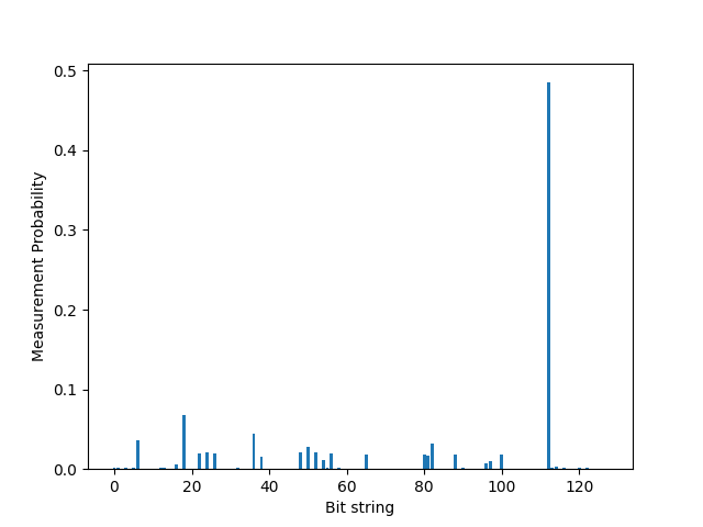
The state \(|112\rangle = |1110000\rangle\) occurs with highest probability. This corresponds to nodes \(0\), \(1\), and \(2\) of the graph, which is the maximum clique! We have successfully combined FALQON and QAOA to solve a combinatorial optimization problem 🎉.

References

Magann, A. B., Rudinger, K. M., Grace, M. D., & Sarovar, M. (2021). Feedback-based quantum optimization. arXiv preprint arXiv:2103.08619.

About the authors

David Wakeham

David's elements formed from exploding stars billions of years ago but self-organized into a human more recently. He has a background in string theory and particle physics, but decided his life would be better spent making colourful widgets. His personal website is hapax.github.io.

Jack Ceroni

Jack is currently a second-year undergraduate student at the University of Toronto, pursuing a degree in pure mathematics. Broadly, his interests are related to simulating quantum systems with quantum computers, mathematical abstraction, and philosophy.

demos/tutorial_falqon

 

Download Python script

 

Download Notebook

 

View on GitHub