Note
Click here to download the full example code
Quantum analytic descent
Authors: Elies Gil-Fuster, David Wierichs (Xanadu Residents) — Posted: 30 June 2021. Last updated: 18 November 2021
One of the main problems of many-body physics is that of finding the ground state and ground state energy of a given Hamiltonian. The Variational Quantum Eigensolver (VQE) combines smart circuit design with gradient-based optimization to solve this task. Several practical demonstrations have shown how near-term quantum devices may be suitable for VQE and other variational quantum algorithms. One issue for such an approach, though, is that the optimization landscape is non-convex, so reaching a good enough local minimum quickly requires hundreds or thousands of update steps. This is problematic because computing gradients of the cost function on a quantum computer is inefficient when it comes to circuits with many parameters.
At the same time, we have a good understanding of the local shape of the cost landscape around any reference point. Cashing in on this, the authors of the Quantum Analytic Descent paper 1 propose an algorithm that constructs a classical model which approximates the landscape, so that the gradients can be calculated on a classical computer, which is much cheaper. In order to build the classical model, we need to use the quantum device to evaluate the cost function on (a) a reference point \(\boldsymbol{\theta}_0\), and (b) a number of points shifted away from \(\boldsymbol{\theta}_0\). With the cost values at these points, we can build the classical model that approximates the landscape.
In this demo, you will learn how to implement Quantum Analytic Descent using PennyLane. In addition, you will look under the hood of the constructed models and the optimization steps carried out by the algorithm. So: sit down, relax, and enjoy your optimization!
Optimization progress with Quantum Analytic Descent.
VQEs give rise to trigonometric cost functions
When we talk about VQEs we have a quantum circuit with \(n\) qubits in mind, which are typically initialized in the base state \(|0\rangle\). The body of the circuit is a variational form \(V(\boldsymbol{\theta})\) – a fixed architecture of quantum gates parametrized by an array of real-valued parameters \(\boldsymbol{\theta}\in\mathbb{R}^m\). After the variational form, the circuit ends with the measurement of a chosen observable \(\mathcal{M}\), based on the problem we are trying to solve.
The idea in VQE is to fix a variational form such that the expected value of the measurement relates to the energy of an interesting Hamiltonian:
We want to find the lowest possible energy the system can attain; this corresponds to running an optimization program to find the \(\boldsymbol{\theta}\) that minimizes the function above.
If the gates in the variational form are restricted to be Pauli rotations, then the cost function is a sum of multilinear trigonometric terms in each of the parameters. That’s a scary sequence of words! What it means is that if we look at \(E(\boldsymbol{\theta})\) but we focus only on one of the parameters, say \(\theta_i\), then we can write the functional dependence as a linear combination of three functions: \(1\), \(\sin(\theta_i)\), and \(\cos(\theta_i)\). That is, for each parameter \(\theta_i\) there exist \(a_i\), \(b_i\), and \(c_i\) such that the cost can be written as
All parameters but \(\theta_i\) are absorbed in the coefficients \(a_i\), \(b_i\) and \(c_i\). Another technique using this structure of \(E(\boldsymbol{\theta})\) are the Rotosolve/Rotoselect algorithms 2 for which there also is a PennyLane demo.
Let’s look at a toy example to illustrate this structure of the cost function.
import pennylane as qml
from pennylane import numpy as np
import matplotlib.pyplot as plt
import warnings

warnings.filterwarnings("ignore")

np.random.seed(0)

# Create a device with 2 qubits.
dev = qml.device("default.qubit", wires=2)

# Define the variational form V and observable M and combine them into a QNode.
@qml.qnode(dev, diff_method="parameter-shift", max_diff=2)
def circuit(parameters):
    qml.RX(parameters[0], wires=0)
    qml.RX(parameters[1], wires=1)
    return qml.expval(qml.PauliZ(0) @ qml.PauliZ(1))
Let us now look at how the energy value depends on each of the two parameters alone. For that, we just fix one parameter and show the cost when varying the other one:
# Create 1D sweeps through parameter space with the other parameter fixed.
num_samples = 50

# Fix a parameter position.
parameters = np.array([3.3, 0.5], requires_grad=True)

theta_func = np.linspace(0, 2 * np.pi, num_samples)
C1 = [circuit(np.array([theta, parameters[1]])) for theta in theta_func]
C2 = [circuit(np.array([parameters[0], theta])) for theta in theta_func]

# Show the sweeps.
fig, ax = plt.subplots(1, 1, figsize=(4, 3))
ax.plot(theta_func, C1, label="$E(\\theta, 0.5)$", color="r")
ax.plot(theta_func, C2, label="$E(3.3, \\theta)$", color="orange")
ax.set_xlabel("$\\theta$")
ax.set_ylabel("$E$")
ax.legend()
plt.tight_layout()

# Create a 2D grid and evaluate the energy on the grid points.
# We cut out a part of the landscape to increase clarity.
X, Y = np.meshgrid(theta_func, theta_func)
Z = np.zeros_like(X)
for i, t1 in enumerate(theta_func):
    for j, t2 in enumerate(theta_func):
        # Cut out the viewer-facing corner
        if (2 * np.pi - t2) ** 2 + t1 ** 2 > 4:
            Z[i, j] = circuit([t1, t2])
        else:
            X[i, j] = Y[i, j] = Z[i, j] = np.nan

# Show the energy landscape on the grid.
fig, ax = plt.subplots(1, 1, subplot_kw={"projection": "3d"}, figsize=(4, 4))
surf = ax.plot_surface(X, Y, Z, label="$E(\\theta_1, \\theta_2)$", alpha=0.7, color="#209494")
line1 = ax.plot(
    [parameters[1]] * num_samples,
    theta_func,
    C1,
    label="$E(\\theta_1, \\theta_2^{(0)})$",
    color="r",
    zorder=100,
)
line2 = ax.plot(
    theta_func,
    [parameters[0]] * num_samples,
    C2,
    label="$E(\\theta_1^{(0)}, \\theta_2)$",
    color="orange",
    zorder=100,
)
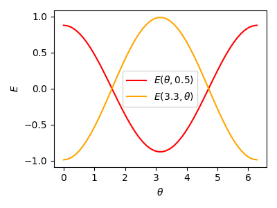
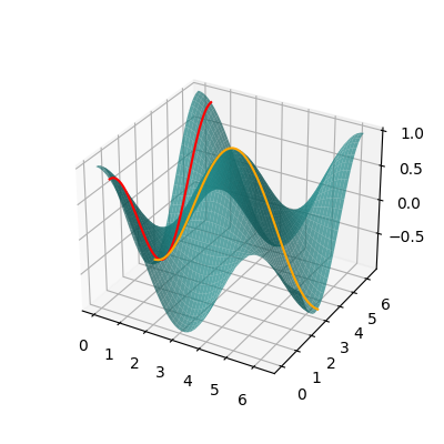
Of course this is an overly simplified example, but the key take-home message so far is: if the variational parameters feed into Pauli rotations, the energy landscape is a multilinear combination of trigonometric functions. What is a good thing about trigonometric functions? That’s right! We have studied them since high school and know how their graphs look.
The QAD strategy
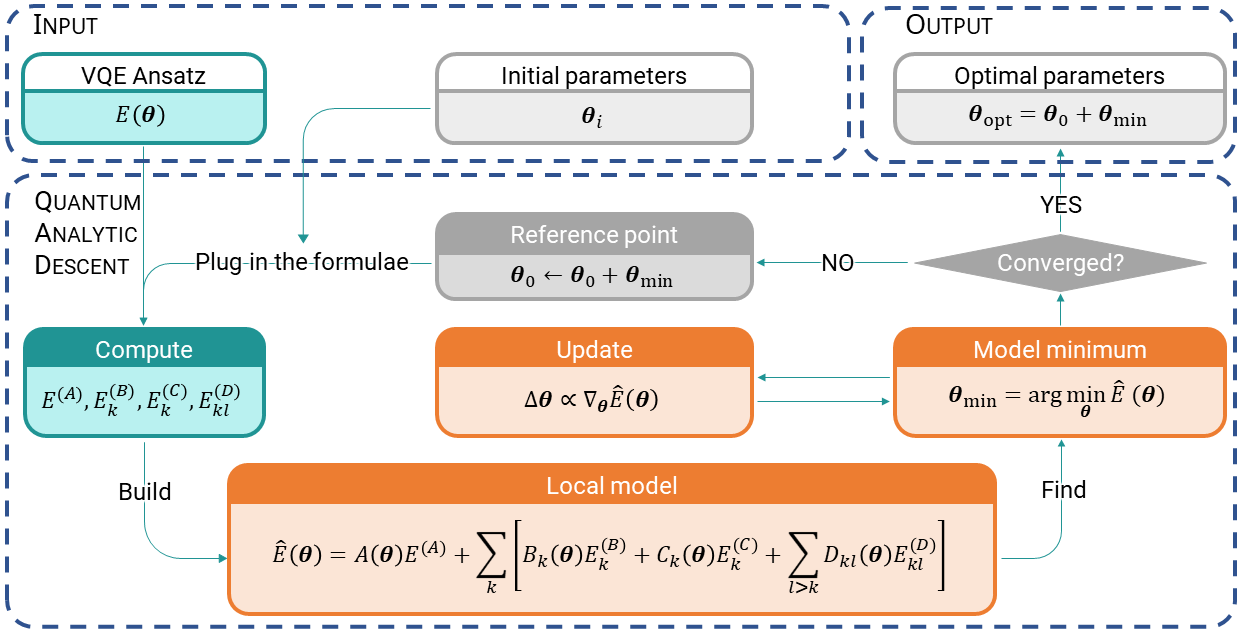
By now we know how the energy landscape looks for a small example. Scaling this up to more parameters would quickly become unfeasible because we need to query a quantum computer for every combination of parameter values. The secret ingredient of this sauce is that we only need to build an approximate classical model. Using an approximate classical model has one feature and one bug. The feature: it is cheap to construct. The bug: well, it’s only approximate, so we cannot rely on it fully. And one extra feature (you didn’t see that coming, did you?): if the reference point about which we build the classical model is a true local minimum, then it will be a local minimum of the classical model too. And that is the key! Given a reference point, we use the classical model to find a point that’s closer to the true minimum, and then use that point as reference for a new model! This is what is called Quantum Analytic Descent (QAD), and if you are fine not knowing yet what all the symbols mean, here’s its pseudo-algorithm:
Set an initial reference point \(\boldsymbol{\theta}_0\).
Build the model \(\hat{E}(\boldsymbol{\theta})\approx E(\boldsymbol{\theta}_0+\boldsymbol{\theta})\) at this point.
Find the minimum \(\boldsymbol{\theta}_\text{min}\) of the model.
Set \(\boldsymbol{\theta}_0+\boldsymbol{\theta}_\text{min}\) as the new reference point \(\boldsymbol{\theta}_0\), go back to Step 2.
After convergence or a fixed number of models built, output the last minimum \(\boldsymbol{\theta}_\text{opt}=\boldsymbol{\theta}_0+\boldsymbol{\theta}_\text{min}\).
Computing a classical model
Knowing how the cost looks when restricted to only one parameter (see the plot above), nothing keeps us in theory from constructing a perfect classical model. The only thing we need to do is write down a general multilinear trigonometric polynomial and determine its coefficients. Simple, right? Well, for \(m\) parameters, there would be \(3^m\) coefficients to estimate, which gives us the ever-dreaded exponential scaling. Although conceptually simple, building an exact model would require exponentially many resources, and that’s a no-go. What can we do, then? The authors of QAD propose building an imperfect model. This makes all the difference—they use a classical model that is accurate only in a region close to a given reference point, and that delivers good results for the optimization!
Function expansions
What do we usually do when we want to approximate something in a region near to a reference point? Correct! We use a Taylor expansion! But what if we told you there is a better option for the case at hand? In the QAD paper, the authors state that a trigonometric expansion up to second order is already a sound model candidate. Let’s recap such expansions.
Taylor expansion vs. Trigonometric expansion
In spirit, a trigonometric expansion and a Taylor expansion are not that different: both are linear combinations of some basis functions, where the coefficients of the sum take very specific values usually related to the derivatives of the function we want to approximate. The difference between Taylor’s and a trigonometric expansion is mainly what basis of functions we take. In Calculus I we learned that a Taylor series in one variable \(x\) uses the integer powers of the variable namely \(\{1, x, x^2, x^3, \ldots\}\), in short \(\{x^n\}_{n\in\mathbb{N}}\):
A trigonometric expansion instead uses a different basis, also for one variable: \(\{1, \sin(x), \cos(x), \sin(2x), \cos(2x), \ldots\}\), which we could call the set of trigonometric monomials with integer frequency, or in short \(\{\sin(nx),\cos(nx)\}_{n\in\mathbb{N}}\):
For higher-dimensional variables we have to take products of the basis functions of each coordinate, i.e., of monomials or trigonometric monomials respectively. This does lead to an exponentially increasing number of terms, but if we chop the series soon enough it will not get too much out of hand. The proposal here is to only go up to second order terms, so we are safe.
Expanding in adapted trigonometric polynomials
One important aspect in which trigonometric series differ from regular expansions is that there is not a clear separation between what terms contribute to each order of the expansion (due to the fact that all derivatives of sine and cosine are non-zero in general). Because of this, we group the terms by their leading order contribution, and in the following table write them next to their non-trigonometric analogues. All chosen trigonometric monomials have leading order coefficient \(1\) and they all differ in their leading order contribution.
Order |
Trigonometric monomial |
Taylor monomial |
|---|---|---|
0 |
\(A(\boldsymbol{\theta})= \prod_{i=1}^m \cos\left(\frac{\theta_i}{2}\right)^2\) |
\(1\) |
1 |
\(B_k(\boldsymbol{\theta}) = 2\cos\left(\frac{\theta_k}{2}\right)\sin\left(\frac{\theta_k}{2}\right)\prod_{i\neq k} \cos\left(\frac{\theta_i}{2}\right)^2\) |
\(x_k\) |
2 |
\(C_k(\boldsymbol{\theta}) = 2\sin\left(\frac{\theta_k}{2}\right)^2\prod_{i\neq k} \cos\left(\frac{\theta_i}{2}\right)^2\) |
\(x_k^2\) |
2 |
\(D_{kl}(\boldsymbol{\theta}) = 4\sin\left(\frac{\theta_k}{2}\right)\cos\left(\frac{\theta_k}{2}\right)\sin\left(\frac{\theta_l}{2}\right)\cos\left(\frac{\theta_l}{2}\right)\prod_{i\neq k,l} \cos\left(\frac{\theta_i}{2}\right)^2\) |
\(x_kx_l\) |
Those are really large terms compared to a Taylor series! However, you may have noticed all of those terms have large parts in common. Indeed, we can rewrite the longer ones in a shorter way which is more decent to look at:
With that, we know what type of terms we should expect to encounter in our local classical model: the model we want to construct is a linear combination of the functions \(A(\boldsymbol{\theta})\), \(B_k(\boldsymbol{\theta})\) and \(C_k(\boldsymbol{\theta})\) for each parameter, and \(D_{kl}(\boldsymbol{\theta})\) for every pair of different parameters \((\theta_k,\theta_l)\).
Computing the expansion coefficients
We can now use the derivatives of the function we are approximating to obtain the coefficients of the linear combination. As the terms we include in the expansion have leading orders \(0\), \(1\) and \(2\), these derivatives are \(E(\boldsymbol{\theta})\), \(\partial E(\boldsymbol{\theta})/\partial \theta_k\), \(\partial^2 E(\boldsymbol{\theta})/\partial\theta_k^2\), and \(\partial^2 E(\boldsymbol{\theta})/\partial \theta_k\partial\theta_l\). However, the trigonometric polynomials may contain multiple orders in \(\boldsymbol{\theta}\). For example, both \(A(\boldsymbol{\theta})\) and \(C_k(\boldsymbol{\theta})\) contribute to the second order, so we have to account for this in the coefficient of \(\partial^2 E(\boldsymbol{\theta})/\partial \theta_k^2\). We can name the different coefficients (including the function value itself) accordingly to how we named the terms in the series:
In PennyLane, computing the gradient of a cost function with respect to an array of parameters can be easily done with the parameter-shift rule. By iterating the rule, we can obtain the second derivatives – the Hessian (see for example 3). Let us implement a function that does just that and prepares the coefficients \(E^{(A/B/C/D)}\):
def get_model_data(fun, params):
    """Computes the coefficients for the classical model, E^(A), E^(B), E^(C), and E^(D)."""
    num_params = len(params)

    # E_A contains the energy at the reference point
    E_A = fun(params)

    # E_B contains the gradient.
    E_B = qml.grad(fun)(params)

    hessian = qml.jacobian(qml.grad(fun))(params)

    # E_C contains the slightly adapted diagonal of the Hessian.
    E_C = np.diag(hessian) + E_A / 2

    # E_D contains the off-diagonal parts of the Hessian.
    # We store each pair (k, l) only once, namely the upper triangle.
    E_D = np.triu(hessian, 1)

    return E_A, E_B, E_C, E_D
Let’s test our brand-new function for the circuit from above, at a random parameter position:
parameters = np.random.random(2, requires_grad=True) * 2 * np.pi
print(f"Random parameters (params): {parameters}")
coeffs = get_model_data(circuit, parameters)
print(
    f"Coefficients at params:",
    f" E_A = {coeffs[0]}",
    f" E_B = {coeffs[1]}",
    f" E_C = {coeffs[2]}",
    f" E_D = {coeffs[3]}",
    sep="\n",
)
Out:
Random parameters (params): [3.44829694 4.49366732]
Coefficients at params:
 E_A = 0.20685619228993007
 E_B = [-0.06551083 -0.9306212 ]
 E_C = [-0.1034281 -0.1034281]
 E_D = [[0.         0.29472535]
 [0.         0.        ]]
The classical model (finally!)
Bringing all of the above ingredients together, we have the following gorgeous trigonometric expansion up to second order:
Let us now take a few moments to breath deeply and admire the entirety of it. On the one hand, we have the \(A\), \(B_k\), \(C_k\), and \(D_{kl}\) functions, which we said are the basis functions of the expansion. On the other hand we have the real-valued coefficients \(E^{(A/B/C/D)}\) for the previous functions which are nothing but the derivatives in the corresponding input components. Combining them yields the trigonometric expansion, which we implement with another function:
def model_cost(params, E_A, E_B, E_C, E_D):
    """Compute the model cost for relative parameters and given model data."""
    A = np.prod(np.cos(0.5 * params) ** 2)

    # For the other terms we only compute the prefactor relative to A
    B_over_A = 2 * np.tan(0.5 * params)
    C_over_A = B_over_A ** 2 / 2
    D_over_A = np.outer(B_over_A, B_over_A)

    all_terms_over_A = [
        E_A,
        np.dot(E_B, B_over_A),
        np.dot(E_C, C_over_A),
        np.dot(B_over_A, E_D @ B_over_A),
    ]

    cost = A * np.sum(all_terms_over_A)

    return cost


# Compute the circuit at parameters (This value is also stored in E_A=coeffs[0])
E_original = circuit(parameters)
# Compute the model at parameters by plugging in relative parameters 0.
E_model = model_cost(np.zeros_like(parameters), *coeffs)
print(
    f"The cost function at parameters:",
    f"  Model:    {E_model}",
    f"  Original: {E_original}",
    sep="\n",
)
# Check that coeffs[0] indeed is the original energy and that the model is correct at 0.
print(f"E_A and E_original are the same: {coeffs[0]==E_original}")
print(f"E_model and E_original are the same: {E_model==E_original}")
Out:
The cost function at parameters:
  Model:    0.20685619228993007
  Original: 0.20685619228993007
E_A and E_original are the same: True
E_model and E_original are the same: True
As we can see, the model reproduces the correct energy at the parameter position \(\boldsymbol{\theta}_0\) at which we constructed it (again note how the input parameters of the model are relative to the reference point such that \(\hat{E}(0)=E(\boldsymbol{\theta}_0)\) is satisfied). When we move away from \(\boldsymbol{\theta}_0\), the model starts to deviate, as it is an approximation after all:
# Obtain a random shift away from parameters
shift = 0.1 * np.random.random(2)
print(f"Shift parameters by the vector {np.round(shift, 4)}.")
new_parameters = parameters + shift
# Compute the cost function and the model at the shifted position.
E_original = circuit(new_parameters)
E_model = model_cost(shift, *coeffs)
print(
    f"The cost function at parameters:",
    f"  Model:    {E_model}",
    f"  Original: {E_original}",
    sep="\n",
)
print(f"E_model and E_original are the same: {E_model==E_original}")
Out:
Shift parameters by the vector [0.0603 0.0545].
The cost function at parameters:
  Model:    0.15256055642369634
  Original: 0.15260964605159766
E_model and E_original are the same: False
Note
Counting parameters and evaluations
How many parameters does our model have? In the following table we count them for an \(m\)-dimensional input variable \(\boldsymbol{\theta}=(\theta_1,\ldots,\theta_m)\):
Number of coefficients |
Number of circuit evaluations |
|
|---|---|---|
\(E^{(A)}\) |
\(1\) |
\(1\) |
\(E^{(B)}\) |
\(m\) |
\(2m\) |
\(E^{(C)}\) |
\(m\) |
\(m\) |
\(E^{(D)}\) |
\(\frac{m(m-1)}{2}\) |
\(4\frac{m(m-1)}{2}\) |
Total: |
\(\frac{m^2}{2}+\frac{3m}{2}+1\) |
\(2m^2+m+1\) |
So there we go! We only need polynomially many parameters and circuit evaluations. This is much cheaper than the \(3^m\) we would need if we naively tried to construct the cost landscape exactly, without chopping after second order.
Now this should be enough theory, so let’s visualize the model that results from our trigonometric expansion.
We’ll use the coefficients and the model_cost function from above and sample a new random parameter position.
from mpl_toolkits.mplot3d import Axes3D
from itertools import product
# We actually make the plotting a function because we will reuse it below.
def plot_cost_and_model(f, model, params, shift_radius=5 * np.pi / 8, num_points=20):
"""Plot a function and a model of the function as well as its deviation."""
coords = np.linspace(-shift_radius, shift_radius, num_points)
X, Y = np.meshgrid(coords + params[0], coords + params[1])
# Compute the original cost function and the model on the grid.
Z_original = np.array([[f(params + np.array([t1, t2])) for t2 in coords] for t1 in coords])
Z_model = np.array([[model(np.array([t1, t2])) for t2 in coords] for t1 in coords])
# Prepare sampled points for plotting rods.
shifts = [-np.pi / 2, 0, np.pi / 2]
samples = []
for s1, s2 in product(shifts, repeat=2):
shifted_params = params + np.array([s1, s2])
samples.append([*(params+np.array([s2, s1])), f(shifted_params)])
# Display landscapes incl. sampled points and deviation.
alpha = 0.6
fig, (ax0, ax1, ax2) = plt.subplots(1, 3, subplot_kw={"projection": "3d"}, figsize=(10, 4))
green = "#209494"
orange = "#ED7D31"
red = "xkcd:brick red"
surf = ax0.plot_surface(X, Y, Z_original, color=green, alpha=alpha)
ax0.set_title("Original energy and samples")
ax1.plot_surface(X, Y, Z_model, color=orange, alpha=alpha)
ax1.set_title("Model energy")
ax2.plot_surface(X, Y, Z_original - Z_model, color=red, alpha=alpha)
ax2.set_title("Deviation")
for s in samples:
ax0.plot([s[0]] * 2, [s[1]] * 2, [np.min(Z_original) - 0.2, s[2]], color="k")
for ax, z in zip((ax0, ax1), (f(params), model(0 * params))):
ax.plot([params[0]] * 2, [params[1]] * 2, [np.min(Z_original) - 0.2, z], color="k")
ax.scatter([params[0]], [params[1]], [z], color="k", marker="o")
plt.tight_layout(pad=2, w_pad=2.5)
# Get some fresh random parameters and the model coefficients
parameters = np.random.random(2, requires_grad=True) * 2 * np.pi
coeffs = get_model_data(circuit, parameters)
# Define a mapped model that has the model coefficients fixed.
mapped_model = lambda params: model_cost(params, *coeffs)
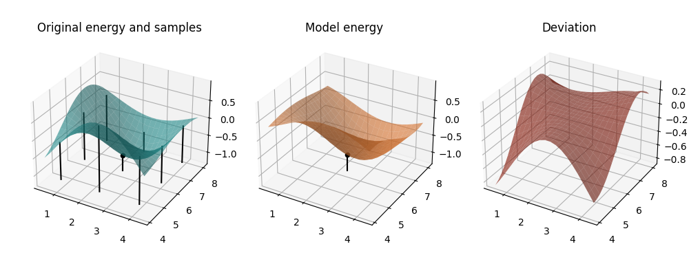
plot_cost_and_model(circuit, mapped_model, parameters)
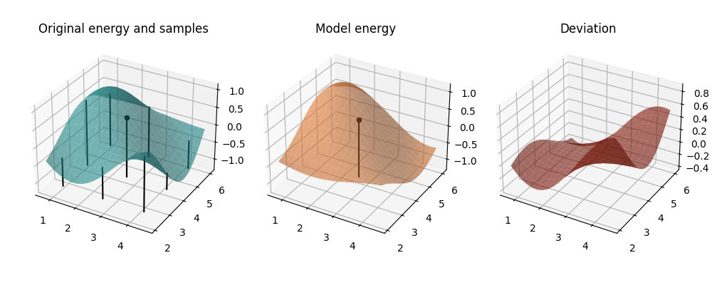
In the first two plots, we see the true landscape, and the approximate model. The vertical rods indicate the points at which the original cost function was evaluated in order to obtain the model coefficients (we skip the additional evaluations for \(E^{(C)}\), though, for clarity of the plot). The rod with the bead on top indicates the reference point around which the model is built and at which it coincides with the original cost function up to second order. This is underlined in the third plot, where we see the difference between the model and true landscapes. Around the reference point the difference is very small and changes very slowly, only growing significantly for large simultaneous perturbations in both parameters. This already hints at the value of the model for local optimization.
Quantum Analytic Descent
The underlying idea we will now try to exploit for optimization in VQEs is the following: if we can model the cost around the reference point well enough, we will be able to find a rough estimate of where the minimum of the landscape is. Granted, our model represents the true landscape less accurately the further we go away from the reference point \(\boldsymbol{\theta}_0\), but nonetheless the minimum of the model will bring us much closer to the minimum of the true cost than a random choice. Recall the complete strategy from above:
Set an initial reference point \(\boldsymbol{\theta}_0\).
Build the model \(\hat{E}(\boldsymbol{\theta})\approx E(\boldsymbol{\theta}_0+\boldsymbol{\theta})\) at this point.
Find the minimum \(\boldsymbol{\theta}_\text{min}\) of the model.
Set \(\boldsymbol{\theta}_0+\boldsymbol{\theta}_\text{min}\) as the new reference point \(\boldsymbol{\theta}_0\), go back to Step 2.
After convergence or a fixed number of models built, output the last minimum \(\boldsymbol{\theta}_\text{opt}=\boldsymbol{\theta}_0+\boldsymbol{\theta}_\text{min}\).
This provides an iterative strategy which will take us to a good enough solution in fewer iterations than, for example, regular stochastic gradient descent (SGD). The procedure of Quantum Analytic Descent is also shown in the following flowchart. Note that the minimization of the model in Step 3 is carried out via an inner optimization loop.
Using the functions from above, we now can implement the loop between Steps 2 and 4. Indeed, for a relatively small number of iterations we should already find a low enough value. If we look back at the circuit we defined, we notice that we are measuring the observable
which has the eigenvalues \(1\) and \(-1\). This means our function is bounded and takes values in the range \([-1,1]\), so that the global minimum should be around \(-1\) if our circuit is expressive enough. Let’s try it and apply the full optimization strategy:
import copy

# Set the number of iterations of Steps 2, 3, and 4
N_iter_outer = 3
N_iter_inner = 50

past_coeffs = []
past_parameters = []
circuit_log = [circuit(parameters)]
model_logs = []

for iter_outer in range(N_iter_outer):
    # Model building phase of outer iteration - step 2.
    coeffs = get_model_data(circuit, parameters)
    past_coeffs.append(copy.deepcopy(coeffs))
    past_parameters.append(parameters.copy())
    # Map the model to be only depending on the parameters, not the coefficients.
    mapped_model = lambda params: model_cost(params, *coeffs)

    if iter_outer == 0:
        print(f"True energy at initial parameters: {np.round(coeffs[0], decimals=4)}\n")

    opt = qml.AdamOptimizer(0.05)
    # Recall that the parameters of the model are relative coordinates.
    # Correspondingly, we initialize at 0, not at parameters.
    relative_parameters = np.zeros_like(parameters, requires_grad=True)
    model_log = [mapped_model(relative_parameters)]
    print(f"-Iteration {iter_outer+1}-")

    # Run the optimizer for N_iter_inner epochs - Step 3.
    for iter_inner in range(N_iter_inner):
        relative_parameters = opt.step(mapped_model, relative_parameters)
        circuit_log.append(circuit(parameters + relative_parameters))
        model_log.append(mapped_model(relative_parameters))
        if (iter_inner + 1) % 50 == 0:
            E_model = mapped_model(relative_parameters)
            print(
                f"Epoch {iter_inner+1:4d}: Model cost = {np.round(E_model, 4)}",
                f" at relative parameters {np.round(relative_parameters, 4)}",
            )

    # Store the relative parameters that minimize the model by adding the shift - Step 4.
    parameters += relative_parameters
    E_original = circuit(parameters)
    print(f"True energy at the minimum of the model: {E_original}")
    print(f"New reference parameters: {np.round(parameters, 4)}\n")
    model_logs.append(model_log)
Out:
True energy at initial parameters: 0.5398

-Iteration 1-
Epoch   50: Model cost = -0.7981  at relative parameters [-0.2397  2.0158]
True energy at the minimum of the model: -0.7358296722728775
New reference parameters: [2.4222 6.0741]

-Iteration 2-
Epoch   50: Model cost = -1.0084  at relative parameters [0.6908 0.2794]
True energy at the minimum of the model: -0.997122597160568
New reference parameters: [3.113  6.3535]

-Iteration 3-
Epoch   50: Model cost = -1.0  at relative parameters [ 0.0272 -0.0685]
True energy at the minimum of the model: -0.9999975843757783
New reference parameters: [3.1403 6.285 ]
This looks great! Quantum Analytic Descent found the minimum.
Inspecting the models
Let us take a look at the intermediate models QAD built:
mapped_model = lambda params: model_cost(params, *past_coeffs[0])
plot_cost_and_model(circuit, mapped_model, past_parameters[0])

Iteration 1: We see the cost function and the model around our starting point. This is the same as the plot before.
mapped_model = lambda params: model_cost(params, *past_coeffs[1])
plot_cost_and_model(circuit, mapped_model, past_parameters[1])
Iteration 2: Now we observe the model better resembles the original landscape. In addition, the minimum of the model is within the displayed range – we’re getting closer.
mapped_model = lambda params: model_cost(params, *past_coeffs[2])
plot_cost_and_model(circuit, mapped_model, past_parameters[2])
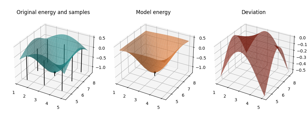
Iteration 3: Both the model and the original cost function now show a minimum close to our parameter position— Quantum Analytic Descent converged. Note how the larger deviations of the model close to the boundaries are not a problem at all because we only use the model in the central area in which both the original energy and the model form a convex bowl and the deviation plateaus at zero.
Optimization behaviour
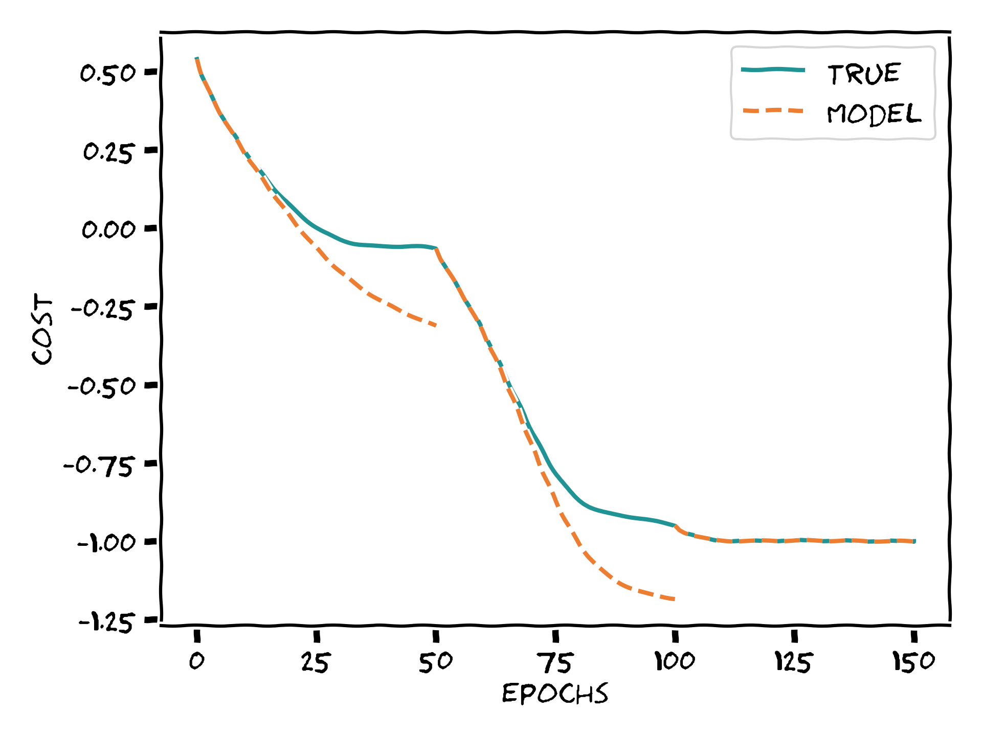
If we pay close attention to the values printed during the optimization, we can identify a curious phenomenon. At the last epochs within some iterations, the model cost goes beyond \(-1\). Could we visualize this behavior more clearly, please?
fig, ax = plt.subplots(1, 1, figsize=(6, 4))
ax.plot(circuit_log, color="#209494", label="True")
for i in range(N_iter_outer):
    x = range(i * N_iter_inner, (i + 1) * N_iter_inner + 1)
    (line,) = ax.plot(x, model_logs[i], ls="--", color="#ED7D31")
    if i == 0:
        line.set_label("Model")
ax.plot([0, N_iter_outer * N_iter_inner], [-1.0, -1.0], lw=0.6, color="0.6", label="Solution")
ax.set_xlabel("epochs")
ax.set_ylabel("cost")
leg = ax.legend()
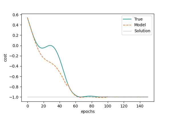
Each of the orange lines corresponds to minimizing the model constructed at a different reference point. We can now more easily appreciate the phenomenon we just described: towards the end of each “outer” optimization step, the model cost can potentially be significantly lower than the true cost. Once the true cost itself approaches the absolute minimum, this means the model cost can overstep the allowed range. Wasn’t this forbidden? You guys told us the function could only take values in \([-1,1]\) >:@ Yes, but careful! While the true cost values are bounded, that does not mean the ones of the model are! Notice also how this only happens at the first stages of analytic descent.
Bringing together a few chords we have touched so far: once we fix a reference value, the further we go from it, the less accurate our model becomes. Thus, if we start far off from the true minimum, it can happen that our model exaggerates how steep the landscape is and then the model minimum lies lower than that of the true cost. We see how values exiting the allowed range of the true cost function does not have an impact on the overall optimization.
In this demo we’ve seen how to implement the Quantum Analytic Descent algorithm using PennyLane for a toy example of a Variational Quantum Eigensolver. By making extensive use of 3D plots we have also tried to illustrate exactly what is going on in both the true cost landscape and the trigonometric expansion approximation. Recall we wanted to avoid working on the true landscape itself because we can only access it via very costly quantum computations. Instead, a fixed number of runs on the quantum device for a few iterations allowed us to construct a classical model on which we performed (cheap) classical optimization.
And that was it! Thanks for coming to our show. Don’t forget to fasten your seat belts on your way home! It was a pleasure having you here today.
References
- 1
Balint Koczor, Simon Benjamin. “Quantum Analytic Descent”. arXiv preprint arXiv:2008.13774.
- 2
Mateusz Ostaszewski, Edward Grant, Marcello Benedetti. “Structure optimization for parameterized quantum circuits”. arXiv preprint arXiv:1905.09692.
- 3
Andrea Mari, Thomas R. Bromley, Nathan Killoran. “Estimating the gradient and higher-order derivatives on quantum hardware”. Phys. Rev. A 103, 012405, 2021. arXiv preprint arXiv:2008.06517.
About the authors

Elies Gil-Fuster

David Wierichs
Total running time of the script: ( 0 minutes 7.583 seconds)