Frugal shot optimization with Rosalin

Author: Josh Izaac — Posted: 19 May 2020. Last updated: 30 January 2023.

In this tutorial we investigate and implement the Rosalin (Random Operator Sampling for Adaptive Learning with Individual Number of shots) from Arrasmith et al. 1. In this paper, a strategy is introduced for reducing the number of shots required when optimizing variational quantum algorithms, by both:

• Frugally adapting the number of shots used per parameter update, and

• Performing a weighted sampling of operators from the cost Hamiltonian.

Note

The Rosalin optimizer is available in PennyLane via the ShotAdaptiveOptimizer.

Background

While a large number of papers in variational quantum algorithms focus on the choice of circuit ansatz, cost function, gradient computation, or initialization method, the optimization strategy—an important component affecting both convergence time and quantum resource dependence—is not as frequently considered. Instead, common ‘out-of-the-box’ classical optimization techniques, such as gradient-free methods (COBLYA, Nelder-Mead), gradient-descent, and Hessian-free methods (L-BFGS) tend to be used.

However, for variational algorithms such as VQE, which involve evaluating a large number of non-commuting operators in the cost function, decreasing the number of quantum evaluations required for convergence, while still minimizing statistical noise, can be a delicate balance.

Recent work has highlighted that ‘quantum-aware’ optimization techniques can lead to marked improvements when training variational quantum algorithms:

• Quantum natural gradient descent by Stokes et al. 2, which takes into account the quantum geometry during the gradient-descent update step.

• The work of Sweke et al. 3, which shows that quantum gradient descent with a finite number of shots is equivalent to stochastic gradient descent, and has guaranteed convergence. Furthermore, combining a finite number of shots with weighted sampling of the cost function terms leads to Doubly stochastic gradient descent.

• The iCANS (individual Coupled Adaptive Number of Shots) optimization technique by Jonas Kuebler et al. 4 adapts the number of shots measurements during training, by maximizing the expected gain per shot.

In this latest result by Arrasmith et al. 1, the idea of doubly stochastic gradient descent has been used to extend the iCANS optimizer, resulting in faster convergence.

Over the course of this tutorial, we will explore their results; beginning first with a demonstration of weighted random sampling of the cost Hamiltonian operators, before combining this with the shot-frugal iCANS optimizer to perform doubly stochastic Rosalin optimization.

Weighted random sampling

Consider a Hamiltonian \(H\) expanded as a weighted sum of operators \(h_i\) that can be directly measured:

\[H = \sum_{i=1}^N c_i h_i.\]

Due to the linearity of expectation values, the expectation value of this Hamiltonian can be expressed as the weighted sum of each individual term:

\[\langle H\rangle = \sum_{i=1}^N c_i \langle h_i\rangle.\]

In the doubly stochastic gradient descent demonstration, we estimated this expectation value by uniformly sampling a subset of the terms at each optimization step, and evaluating each term by using the same finite number of shots \(N\).

However, what happens if we use a weighted approach to determine how to distribute our samples across the terms of the Hamiltonian? In weighted random sampling (WRS), the number of shots used to determine the expectation value \(\langle h_i\rangle\) is a discrete random variable distributed according to a multinomial distribution,

\[S \sim \text{Multinomial}(p_i),\]

with event probabilities

\[p_i = \frac{|c_i|}{\sum_i |c_i|}.\]

That is, the number of shots assigned to the measurement of the expectation value of the \(i\text{th}\) term of the Hamiltonian is drawn from a probability distribution proportional to the magnitude of its coefficient \(c_i\).

To see this strategy in action, consider the Hamiltonian

\[H = 2I\otimes X + 4 I\otimes Z - X\otimes X + 5Y\otimes Y + 2 Z\otimes X.\]

We can solve for the ground state energy using the variational quantum eigensolver (VQE) algorithm.

First, let’s import NumPy and PennyLane, and define our Hamiltonian.

import pennylane as qml
from pennylane import numpy as np

# set the random seed
np.random.seed(4)

coeffs = [2, 4, -1, 5, 2]

obs = [
  qml.PauliX(1),
  qml.PauliZ(1),
  qml.PauliX(0) @ qml.PauliX(1),
  qml.PauliY(0) @ qml.PauliY(1),
  qml.PauliZ(0) @ qml.PauliZ(1)
]

We can now create our quantum device (let’s use the default.qubit simulator).

num_layers = 2
num_wires = 2

# create a device that estimates expectation values using a finite number of shots
non_analytic_dev = qml.device("default.qubit", wires=num_wires, shots=100)

# create a device that calculates exact expectation values
analytic_dev = qml.device("default.qubit", wires=num_wires, shots=None)

Now, let’s set the total number of shots, and determine the probability for sampling each Hamiltonian term.

total_shots = 8000
prob_shots = np.abs(coeffs) / np.sum(np.abs(coeffs))
print(prob_shots)

Out:

[0.14285714 0.28571429 0.07142857 0.35714286 0.14285714]

We can now use SciPy to create our multinomial distributed random variable \(S\), using the number of trials (total shot number) and probability values:

from scipy.stats import multinomial

si = multinomial(n=total_shots, p=prob_shots)

Sampling from this distribution will provide the number of shots used to sample each term in the Hamiltonian:

samples = si.rvs()[0]
print(samples)
print(sum(samples))

Out:

[1191 2262  552 2876 1119]
8000

As expected, if we sum the sampled shots per term, we recover the total number of shots.

Let’s now create our cost function. Recall that the cost function must do the following:

1. It must sample from the multinomial distribution we created above, to determine the number of shots \(s_i\) to use to estimate the expectation value of the ith Hamiltonian term.

2. It then must estimate the expectation value \(\langle h_i\rangle\) by creating the required QNode. For our ansatz, we’ll use the StronglyEntanglingLayers.

3. And, last but not least, estimate the expectation value \(\langle H\rangle = \sum_i c_i\langle h_i\rangle\).

from pennylane.templates.layers import StronglyEntanglingLayers


@qml.qnode(non_analytic_dev, diff_method="parameter-shift", interface="autograd")
def qnode(weights, observable):
    StronglyEntanglingLayers(weights, wires=non_analytic_dev.wires)
    return qml.expval(observable)

def cost(params):
    # sample from the multinomial distribution
    shots_per_term = si.rvs()[0]

    result = 0

    for o, c, s in zip(obs, coeffs, shots_per_term):
        # evaluate the QNode corresponding to
        # the Hamiltonian term, and add it on to our running sum
        result += c * qnode(params, o, shots=int(s))

    return result

Evaluating our cost function with some initial parameters, we can test out that our cost function evaluates correctly.

param_shape = StronglyEntanglingLayers.shape(n_layers=num_layers, n_wires=num_wires)
init_params = np.random.uniform(low=0.0, high=2*np.pi, size=param_shape, requires_grad=True)
print(cost(init_params))

Out:

-0.8395887630997874

Performing the optimization, with the number of shots randomly determined at each optimization step:

opt = qml.AdamOptimizer(0.05)
params = init_params

cost_wrs = []
shots_wrs = []

for i in range(100):
    params, _cost = opt.step_and_cost(cost, params)
    cost_wrs.append(_cost)
    shots_wrs.append(total_shots*i)
    print("Step {}: cost = {} shots used = {}".format(i, cost_wrs[-1], shots_wrs[-1]))

Out:

Step 0: cost = -0.47971271815214855 shots used = 0
Step 1: cost = -1.9358195375281395 shots used = 8000
Step 2: cost = -2.429697191348172 shots used = 16000
Step 3: cost = -3.6308900629353356 shots used = 24000
Step 4: cost = -4.275894772648205 shots used = 32000
Step 5: cost = -5.2697645839743705 shots used = 40000
Step 6: cost = -5.414011202290673 shots used = 48000
Step 7: cost = -5.958619200612785 shots used = 56000
Step 8: cost = -6.589890076928924 shots used = 64000
Step 9: cost = -6.879689304585086 shots used = 72000
Step 10: cost = -7.11044038351491 shots used = 80000
Step 11: cost = -7.441618274754085 shots used = 88000
Step 12: cost = -7.343694305020567 shots used = 96000
Step 13: cost = -7.531129303076952 shots used = 104000
Step 14: cost = -7.3929094864194465 shots used = 112000
Step 15: cost = -7.41913469502728 shots used = 120000
Step 16: cost = -7.484772628807 shots used = 128000
Step 17: cost = -7.2470111788679805 shots used = 136000
Step 18: cost = -7.278243959604719 shots used = 144000
Step 19: cost = -7.21024168219871 shots used = 152000
Step 20: cost = -7.497562843426365 shots used = 160000
Step 21: cost = -7.300503461549561 shots used = 168000
Step 22: cost = -7.502226318725064 shots used = 176000
Step 23: cost = -7.683018234663317 shots used = 184000
Step 24: cost = -7.7122067730786 shots used = 192000
Step 25: cost = -7.502924268040441 shots used = 200000
Step 26: cost = -7.655288657867658 shots used = 208000
Step 27: cost = -7.606898557639433 shots used = 216000
Step 28: cost = -7.625269501080646 shots used = 224000
Step 29: cost = -7.669368776362655 shots used = 232000
Step 30: cost = -7.810865011077598 shots used = 240000
Step 31: cost = -7.679683881569233 shots used = 248000
Step 32: cost = -7.654476847955421 shots used = 256000
Step 33: cost = -7.5211521050495636 shots used = 264000
Step 34: cost = -7.751101012112956 shots used = 272000
Step 35: cost = -7.687077255130304 shots used = 280000
Step 36: cost = -7.736266201334557 shots used = 288000
Step 37: cost = -7.680984283808025 shots used = 296000
Step 38: cost = -7.718561744208679 shots used = 304000
Step 39: cost = -7.67028103083904 shots used = 312000
Step 40: cost = -7.710347919579339 shots used = 320000
Step 41: cost = -7.593136197480478 shots used = 328000
Step 42: cost = -7.810359527538487 shots used = 336000
Step 43: cost = -7.737769438457732 shots used = 344000
Step 44: cost = -7.853027575362733 shots used = 352000
Step 45: cost = -7.87316397259127 shots used = 360000
Step 46: cost = -7.918883946761729 shots used = 368000
Step 47: cost = -7.921546467893382 shots used = 376000
Step 48: cost = -7.71980941701694 shots used = 384000
Step 49: cost = -7.8308057919156155 shots used = 392000
Step 50: cost = -7.8469319373986925 shots used = 400000
Step 51: cost = -7.814094417970937 shots used = 408000
Step 52: cost = -7.805577964490593 shots used = 416000
Step 53: cost = -7.792672651319024 shots used = 424000
Step 54: cost = -7.859279576823298 shots used = 432000
Step 55: cost = -7.920898395551514 shots used = 440000
Step 56: cost = -8.109172247437503 shots used = 448000
Step 57: cost = -7.954949088064669 shots used = 456000
Step 58: cost = -7.840000679159047 shots used = 464000
Step 59: cost = -8.073897469157906 shots used = 472000
Step 60: cost = -8.016380156819022 shots used = 480000
Step 61: cost = -7.749354818376889 shots used = 488000
Step 62: cost = -7.9084244778219634 shots used = 496000
Step 63: cost = -7.911403066159991 shots used = 504000
Step 64: cost = -7.694258154002229 shots used = 512000
Step 65: cost = -8.135637132372215 shots used = 520000
Step 66: cost = -7.880710119461283 shots used = 528000
Step 67: cost = -7.958115647880543 shots used = 536000
Step 68: cost = -7.949005635306886 shots used = 544000
Step 69: cost = -7.815469675932031 shots used = 552000
Step 70: cost = -7.824093391711489 shots used = 560000
Step 71: cost = -7.867760065578605 shots used = 568000
Step 72: cost = -7.931110498889814 shots used = 576000
Step 73: cost = -7.879521348618871 shots used = 584000
Step 74: cost = -7.840075562849998 shots used = 592000
Step 75: cost = -7.866075581377627 shots used = 600000
Step 76: cost = -7.923529733995367 shots used = 608000
Step 77: cost = -7.934656834108851 shots used = 616000
Step 78: cost = -7.894211944790477 shots used = 624000
Step 79: cost = -7.8338507678458065 shots used = 632000
Step 80: cost = -7.7936236744612 shots used = 640000
Step 81: cost = -7.9924846833802 shots used = 648000
Step 82: cost = -7.767589081568244 shots used = 656000
Step 83: cost = -8.036426061542748 shots used = 664000
Step 84: cost = -8.085968623696424 shots used = 672000
Step 85: cost = -7.798674831445482 shots used = 680000
Step 86: cost = -7.771240866851645 shots used = 688000
Step 87: cost = -7.805259795070319 shots used = 696000
Step 88: cost = -7.892488048336198 shots used = 704000
Step 89: cost = -7.894970226892511 shots used = 712000
Step 90: cost = -7.881326529610687 shots used = 720000
Step 91: cost = -8.108673203429863 shots used = 728000
Step 92: cost = -7.907973083754514 shots used = 736000
Step 93: cost = -7.801569622806004 shots used = 744000
Step 94: cost = -7.933400493853428 shots used = 752000
Step 95: cost = -7.8470947907663415 shots used = 760000
Step 96: cost = -7.943261293748337 shots used = 768000
Step 97: cost = -7.818450593894962 shots used = 776000
Step 98: cost = -7.9210182454846425 shots used = 784000
Step 99: cost = -8.111046662059286 shots used = 792000

Let’s compare this against an optimization not using weighted random sampling. Here, we will split the 8000 total shots evenly across all Hamiltonian terms, also known as uniform deterministic sampling.

@qml.qnode(non_analytic_dev, diff_method="parameter-shift", interface="autograd")
def qnode(weights, obs):
    StronglyEntanglingLayers(weights, wires=non_analytic_dev.wires)
    return qml.expval(obs)

def cost(params):
    shots_per_term = int(total_shots / len(coeffs))

    result = 0

    for o, c in zip(obs, coeffs):

        # evaluate the QNode corresponding to
        # the Hamiltonian term, and add it on to our running sum
        result += c * qnode(params, o, shots=shots_per_term)

    return result

opt = qml.AdamOptimizer(0.05)
params = init_params

cost_adam = []
shots_adam = []

for i in range(100):
    params, _cost = opt.step_and_cost(cost, params)
    cost_adam.append(_cost)
    shots_adam.append(total_shots*i)
    print("Step {}: cost = {} shots used = {}".format(i, cost_adam[-1], shots_adam[-1]))

Out:

Step 0: cost = -0.6424999999999998 shots used = 0
Step 1: cost = -1.7650000000000001 shots used = 8000
Step 2: cost = -3.0875 shots used = 16000
Step 3: cost = -3.47875 shots used = 24000
Step 4: cost = -4.405 shots used = 32000
Step 5: cost = -5.126250000000001 shots used = 40000
Step 6: cost = -5.6625 shots used = 48000
Step 7: cost = -5.9837500000000015 shots used = 56000
Step 8: cost = -6.50375 shots used = 64000
Step 9: cost = -6.775 shots used = 72000
Step 10: cost = -6.90625 shots used = 80000
Step 11: cost = -7.165 shots used = 88000
Step 12: cost = -7.39375 shots used = 96000
Step 13: cost = -7.52 shots used = 104000
Step 14: cost = -7.547499999999999 shots used = 112000
Step 15: cost = -7.512499999999999 shots used = 120000
Step 16: cost = -7.155 shots used = 128000
Step 17: cost = -7.534999999999999 shots used = 136000
Step 18: cost = -7.350000000000001 shots used = 144000
Step 19: cost = -7.25625 shots used = 152000
Step 20: cost = -7.3987500000000015 shots used = 160000
Step 21: cost = -7.50875 shots used = 168000
Step 22: cost = -7.50375 shots used = 176000
Step 23: cost = -7.55625 shots used = 184000
Step 24: cost = -7.3374999999999995 shots used = 192000
Step 25: cost = -7.7524999999999995 shots used = 200000
Step 26: cost = -7.6499999999999995 shots used = 208000
Step 27: cost = -7.7524999999999995 shots used = 216000
Step 28: cost = -7.637500000000001 shots used = 224000
Step 29: cost = -7.5512500000000005 shots used = 232000
Step 30: cost = -7.7175 shots used = 240000
Step 31: cost = -7.65625 shots used = 248000
Step 32: cost = -7.998749999999999 shots used = 256000
Step 33: cost = -7.67375 shots used = 264000
Step 34: cost = -7.2962500000000015 shots used = 272000
Step 35: cost = -7.5874999999999995 shots used = 280000
Step 36: cost = -7.74875 shots used = 288000
Step 37: cost = -7.713749999999999 shots used = 296000
Step 38: cost = -7.735 shots used = 304000
Step 39: cost = -7.893750000000001 shots used = 312000
Step 40: cost = -7.57 shots used = 320000
Step 41: cost = -7.7787500000000005 shots used = 328000
Step 42: cost = -7.83 shots used = 336000
Step 43: cost = -7.8475 shots used = 344000
Step 44: cost = -7.82875 shots used = 352000
Step 45: cost = -7.819999999999999 shots used = 360000
Step 46: cost = -7.836250000000001 shots used = 368000
Step 47: cost = -7.786250000000001 shots used = 376000
Step 48: cost = -7.8625 shots used = 384000
Step 49: cost = -7.951250000000001 shots used = 392000
Step 50: cost = -7.958749999999999 shots used = 400000
Step 51: cost = -8.20375 shots used = 408000
Step 52: cost = -7.692500000000001 shots used = 416000
Step 53: cost = -7.8375 shots used = 424000
Step 54: cost = -7.6312500000000005 shots used = 432000
Step 55: cost = -7.828749999999999 shots used = 440000
Step 56: cost = -7.8625 shots used = 448000
Step 57: cost = -8.09125 shots used = 456000
Step 58: cost = -7.70625 shots used = 464000
Step 59: cost = -7.8237499999999995 shots used = 472000
Step 60: cost = -8.03625 shots used = 480000
Step 61: cost = -7.972499999999999 shots used = 488000
Step 62: cost = -7.81 shots used = 496000
Step 63: cost = -7.86375 shots used = 504000
Step 64: cost = -8.045 shots used = 512000
Step 65: cost = -7.80375 shots used = 520000
Step 66: cost = -7.90375 shots used = 528000
Step 67: cost = -7.9025 shots used = 536000
Step 68: cost = -8.01875 shots used = 544000
Step 69: cost = -7.9725 shots used = 552000
Step 70: cost = -8.03625 shots used = 560000
Step 71: cost = -8.09875 shots used = 568000
Step 72: cost = -7.7925 shots used = 576000
Step 73: cost = -7.68 shots used = 584000
Step 74: cost = -7.995 shots used = 592000
Step 75: cost = -7.93625 shots used = 600000
Step 76: cost = -7.74125 shots used = 608000
Step 77: cost = -7.72 shots used = 616000
Step 78: cost = -7.710000000000001 shots used = 624000
Step 79: cost = -7.7125 shots used = 632000
Step 80: cost = -7.7325 shots used = 640000
Step 81: cost = -7.93125 shots used = 648000
Step 82: cost = -7.785 shots used = 656000
Step 83: cost = -7.7625 shots used = 664000
Step 84: cost = -7.6937500000000005 shots used = 672000
Step 85: cost = -8.0525 shots used = 680000
Step 86: cost = -8.06125 shots used = 688000
Step 87: cost = -7.8812500000000005 shots used = 696000
Step 88: cost = -7.973750000000001 shots used = 704000
Step 89: cost = -7.89875 shots used = 712000
Step 90: cost = -7.88 shots used = 720000
Step 91: cost = -7.99875 shots used = 728000
Step 92: cost = -7.86375 shots used = 736000
Step 93: cost = -7.911250000000001 shots used = 744000
Step 94: cost = -7.842500000000001 shots used = 752000
Step 95: cost = -8.00875 shots used = 760000
Step 96: cost = -7.859999999999999 shots used = 768000
Step 97: cost = -7.96375 shots used = 776000
Step 98: cost = -7.772499999999999 shots used = 784000
Step 99: cost = -7.9475 shots used = 792000

Comparing these two techniques:

from matplotlib import pyplot as plt

plt.style.use("seaborn")
plt.plot(shots_wrs, cost_wrs, "b", label="Adam WRS")
plt.plot(shots_adam, cost_adam, "g", label="Adam")

plt.ylabel("Cost function value")
plt.xlabel("Number of shots")
plt.legend()
plt.show()

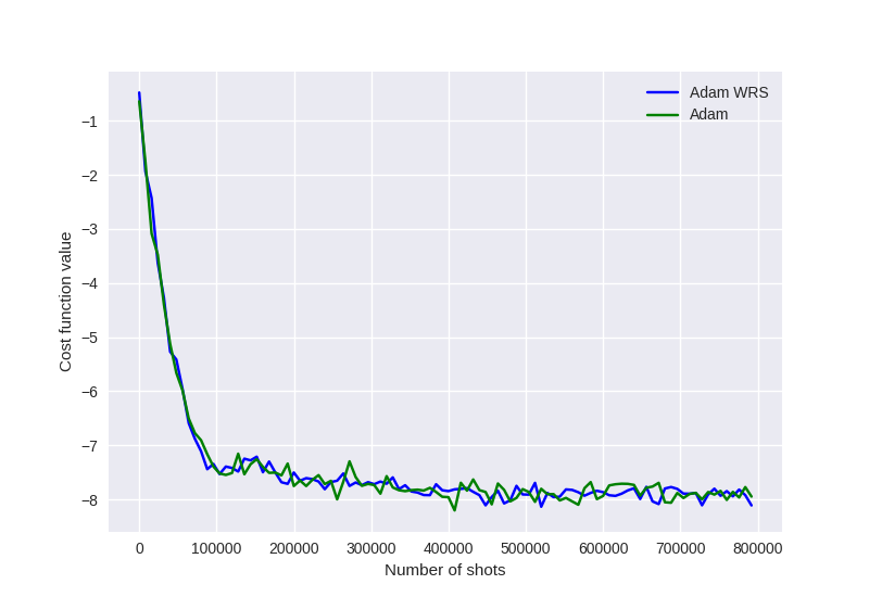
We can see that weighted random sampling performs just as well as the uniform deterministic sampling. However, weighted random sampling begins to show a non-negligible improvement over deterministic sampling for large Hamiltonians with highly non-uniform coefficients. For example, see Fig (3) and (4) of Arrasmith et al. 1, comparing weighted random sampling VQE optimization for both \(\text{H}_2\) and \(\text{LiH}\) molecules.

Note

While not covered here, another approach that could be taken is weighted deterministic sampling. Here, the number of shots is distributed across terms as per

\[s_i = \left\lfloor N \frac{|c_i|}{\sum_i |c_i|}\right\rfloor,\]

where \(N\) is the total number of shots.

Rosalin: Frugal shot optimization

We can see above that both methods optimize fairly well; weighted random sampling converges just as well as evenly distributing the shots across all Hamiltonian terms. However, deterministic shot distribution approaches will always have a minimum shot value required per expectation value, as below this threshold they become biased estimators. This is not the case with random sampling; as we saw in the doubly stochastic gradient descent demonstration, the introduction of randomness allows for as little as a single shot per expectation term, while still remaining an unbiased estimator.

Using this insight, Arrasmith et al. 1 modified the iCANS frugal shot-optimization technique 4 to include weighted random sampling, making it ‘doubly stochastic’.

iCANS optimizer

Two variants of the iCANS optimizer were introduced in Kübler et al., iCANS1 and iCANS2. The iCANS1 optimizer, on which Rosalin is based, frugally distributes a shot budget across the partial derivatives of each parameter, which are computed using the parameter-shift rule. It works roughly as follows:

1. The initial step of the optimizer is performed with some specified minimum number of shots, \(s_{min}\), for all partial derivatives.

2. The parameter-shift rule is then used to estimate the gradient \(g_i\) for each parameter \(\theta_i\), parameters, as well as the variances \(v_i\) of the estimated gradients.

3. Gradient descent is performed for each parameter \(\theta_i\), using the pre-defined learning rate \(\alpha\) and the gradient information \(g_i\):

   \[\theta_i = \theta_i - \alpha g_i.\]

4. The improvement in the cost function per shot, for a specific parameter value, is then calculated via

   \[\gamma_i = \frac{1}{s_i} \left[ \left(\alpha - \frac{1}{2} L\alpha^2\right) g_i^2 - \frac{L\alpha^2}{2s_i}v_i \right],\]

   where:

   • \(L \leq \sum_i|c_i|\) is the bound on the Lipschitz constant of the variational quantum algorithm objective function,

   • \(c_i\) are the coefficients of the Hamiltonian, and

   • \(\alpha\) is the learning rate, and must be bound such that \(\alpha < 2/L\) for the above expression to hold.

5. Finally, the new values of \(s_i\) (shots for partial derivative of parameter \(\theta_i\)) is given by:

   \[s_i = \frac{2L\alpha}{2-L\alpha}\left(\frac{v_i}{g_i^2}\right)\propto \frac{v_i}{g_i^2}.\]

In addition to the above, to counteract the presence of noise in the system, a running average of \(g_i\) and \(s_i\) (\(\chi_i\) and \(\xi_i\) respectively) are used when computing \(\gamma_i\) and \(s_i\).

Note

In classical machine learning, the Lipschitz constant of the cost function is generally unknown. However, for a variational quantum algorithm with cost of the form \(f(x) = \langle \psi(x) | \hat{H} |\psi(x)\rangle\), an upper bound on the Lipschitz constant is given by \(L < \sum_i|c_i|\), where \(c_i\) are the coefficients of \(\hat{H}\) when decomposed into a linear combination of Pauli-operator tensor products.

Rosalin implementation

Let’s now modify iCANS above to incorporate weighted random sampling of Hamiltonian terms — the Rosalin frugal shot optimizer.

Rosalin takes several hyper-parameters:

• min_shots: the minimum number of shots used to estimate the expectations of each term in the Hamiltonian. Note that this must be larger than 2 for the variance of the gradients to be computed.

• mu: The running average constant \(\mu\in[0, 1]\). Used to control how quickly the number of shots recommended for each gradient component changes.

• b: Regularization bias. The bias should be kept small, but non-zero.

• lr: The learning rate. Recall from above that the learning rate must be such that \(\alpha < 2/L = 2/\sum_i|c_i|\).

Since the Rosalin optimizer has a state that must be preserved between optimization steps, let’s use a class to create our optimizer.

class Rosalin:

    def __init__(self, obs, coeffs, min_shots, mu=0.99, b=1e-6, lr=0.07):
        self.obs = obs
        self.coeffs = coeffs

        self.lipschitz = np.sum(np.abs(coeffs))

        if lr > 2 / self.lipschitz:
            raise ValueError("The learning rate must be less than ", 2 / self.lipschitz)

        # hyperparameters
        self.min_shots = min_shots
        self.mu = mu  # running average constant
        self.b = b    # regularization bias
        self.lr = lr  # learning rate

        # keep track of the total number of shots used
        self.shots_used = 0
        # total number of iterations
        self.k = 0
        # Number of shots per parameter
        self.s = np.zeros_like(params, dtype=np.float64) + min_shots

        # Running average of the parameter gradients
        self.chi = None
        # Running average of the variance of the parameter gradients
        self.xi = None

    def estimate_hamiltonian(self, params, shots):
        """Returns an array containing length ``shots`` single-shot estimates
        of the Hamiltonian. The shots are distributed randomly over
        the terms in the Hamiltonian, as per a Multinomial distribution.

        Since we are performing single-shot estimates, the QNodes must be
        set to 'sample' mode.
        """
        rosalin_device = qml.device("default.qubit", wires=num_wires, shots=100)

        # determine the shot probability per term
        prob_shots = np.abs(coeffs) / np.sum(np.abs(coeffs))

        # construct the multinomial distribution, and sample
        # from it to determine how many shots to apply per term
        si = multinomial(n=shots, p=prob_shots)
        shots_per_term = si.rvs()[0]

        results = []

        @qml.qnode(rosalin_device, diff_method="parameter-shift", interface="autograd")
        def qnode(weights, observable):
            StronglyEntanglingLayers(weights, wires=rosalin_device.wires)
            return qml.sample(observable)

        for o, c, p, s in zip(self.obs, self.coeffs, prob_shots, shots_per_term):

            # if the number of shots is 0, do nothing
            if s == 0:
                continue

            # evaluate the QNode corresponding to
            # the Hamiltonian term
            res = qnode(params, o, shots=int(s))

            if s == 1:
                res = np.array([res])

            # Note that, unlike above, we divide each term by the
            # probability per shot. This is because we are sampling one at a time.
            results.append(c * res / p)

        return np.concatenate(results)

    def evaluate_grad_var(self, i, params, shots):
        """Evaluate the gradient, as well as the variance in the gradient,
        for the ith parameter in params, using the parameter-shift rule.
        """
        shift = np.zeros_like(params)
        shift[i] = np.pi / 2

        shift_forward = self.estimate_hamiltonian(params + shift, shots)
        shift_backward = self.estimate_hamiltonian(params - shift, shots)

        g = np.mean(shift_forward - shift_backward) / 2
        s = np.var((shift_forward - shift_backward) / 2, ddof=1)

        return g, s

    def step(self, params):
        """Perform a single step of the Rosalin optimizer."""
        # keep track of the number of shots run
        self.shots_used += int(2 * np.sum(self.s))

        # compute the gradient, as well as the variance in the gradient,
        # using the number of shots determined by the array s.
        grad = []
        S = []

        p_ind = list(np.ndindex(*params.shape))

        for l in p_ind:
            # loop through each parameter, performing
            # the parameter-shift rule
            g_, s_ = self.evaluate_grad_var(l, params, self.s[l])
            grad.append(g_)
            S.append(s_)

        grad = np.reshape(np.stack(grad), params.shape)
        S = np.reshape(np.stack(S), params.shape)

        # gradient descent update
        params = params - self.lr * grad

        if self.xi is None:
            self.chi = np.zeros_like(params, dtype=np.float64)
            self.xi = np.zeros_like(params, dtype=np.float64)

        # running average of the gradient variance
        self.xi = self.mu * self.xi + (1 - self.mu) * S
        xi = self.xi / (1 - self.mu ** (self.k + 1))

        # running average of the gradient
        self.chi = self.mu * self.chi + (1 - self.mu) * grad
        chi = self.chi / (1 - self.mu ** (self.k + 1))

        # determine the new optimum shots distribution for the next
        # iteration of the optimizer
        s = np.ceil(
            (2 * self.lipschitz * self.lr * xi)
            / ((2 - self.lipschitz * self.lr) * (chi ** 2 + self.b * (self.mu ** self.k)))
        )

        # apply an upper and lower bound on the new shot distributions,
        # to avoid the number of shots reducing below min(2, min_shots),
        # or growing too significantly.
        gamma = (
            (self.lr - self.lipschitz * self.lr ** 2 / 2) * chi ** 2
            - xi * self.lipschitz * self.lr ** 2 / (2 * s)
        ) / s

        argmax_gamma = np.unravel_index(np.argmax(gamma), gamma.shape)
        smax = s[argmax_gamma]
        self.s = np.clip(s, min(2, self.min_shots), smax)

        self.k += 1
        return params

Rosalin optimization

We are now ready to use our Rosalin optimizer to optimize the initial VQE problem. But first let’s also create a separate cost function using an ‘exact’ quantum device, so that we can keep track of the exact cost function value at each iteration.

@qml.qnode(analytic_dev, interface="autograd")
def cost_analytic(weights):
    StronglyEntanglingLayers(weights, wires=analytic_dev.wires)
    return qml.expval(qml.Hamiltonian(coeffs, obs))

Creating the optimizer and beginning the optimization:

opt = Rosalin(obs, coeffs, min_shots=10)
params = init_params

cost_rosalin = [cost_analytic(params)]
shots_rosalin = [0]

for i in range(60):
    params = opt.step(params)
    cost_rosalin.append(cost_analytic(params))
    shots_rosalin.append(opt.shots_used)
    print(f"Step {i}: cost = {cost_rosalin[-1]}, shots_used = {shots_rosalin[-1]}")

Out:

Step 0: cost = -4.820380999693453, shots_used = 240
Step 1: cost = -4.937944875992972, shots_used = 336
Step 2: cost = -5.477016391676939, shots_used = 456
Step 3: cost = -5.878302378912973, shots_used = 624
Step 4: cost = -5.7409832352988746, shots_used = 768
Step 5: cost = -5.8684995071744535, shots_used = 960
Step 6: cost = -5.57259761875493, shots_used = 1200
Step 7: cost = -6.038511127131685, shots_used = 1512
Step 8: cost = -7.18783985074634, shots_used = 1944
Step 9: cost = -7.244742040043008, shots_used = 2472
Step 10: cost = -6.955119947427081, shots_used = 3144
Step 11: cost = -7.324280331788419, shots_used = 4176
Step 12: cost = -7.305099179560384, shots_used = 5400
Step 13: cost = -7.241339003277952, shots_used = 6528
Step 14: cost = -7.529075219255001, shots_used = 7632
Step 15: cost = -7.095276433317595, shots_used = 9048
Step 16: cost = -7.607336707435145, shots_used = 10584
Step 17: cost = -7.738585612241668, shots_used = 12624
Step 18: cost = -7.7927004721043005, shots_used = 15288
Step 19: cost = -7.802640154411867, shots_used = 18048
Step 20: cost = -7.765196284526807, shots_used = 20976
Step 21: cost = -7.779379995219436, shots_used = 24264
Step 22: cost = -7.851415989752516, shots_used = 27576
Step 23: cost = -7.829808564028127, shots_used = 31728
Step 24: cost = -7.81374354509188, shots_used = 36264
Step 25: cost = -7.790635224170298, shots_used = 42024
Step 26: cost = -7.887177094048006, shots_used = 48096
Step 27: cost = -7.877872495361853, shots_used = 54744
Step 28: cost = -7.87567921532984, shots_used = 62448
Step 29: cost = -7.855902055330613, shots_used = 71352
Step 30: cost = -7.8844348641017685, shots_used = 80832
Step 31: cost = -7.8916373642127065, shots_used = 90336
Step 32: cost = -7.854723497132753, shots_used = 100680
Step 33: cost = -7.860436984930214, shots_used = 111984
Step 34: cost = -7.885736157831493, shots_used = 123312
Step 35: cost = -7.851714069232079, shots_used = 136632
Step 36: cost = -7.864848529367195, shots_used = 150744
Step 37: cost = -7.875581235645933, shots_used = 166152
Step 38: cost = -7.809686333605919, shots_used = 183240
Step 39: cost = -7.884245542198441, shots_used = 202752
Step 40: cost = -7.889534749964764, shots_used = 221448
Step 41: cost = -7.894948220964509, shots_used = 240192
Step 42: cost = -7.897425239891585, shots_used = 262368
Step 43: cost = -7.879902900295499, shots_used = 285024
Step 44: cost = -7.873122596846599, shots_used = 307704
Step 45: cost = -7.8892855631082845, shots_used = 331272
Step 46: cost = -7.893112373227318, shots_used = 357552
Step 47: cost = -7.878308602523568, shots_used = 385320
Step 48: cost = -7.899236702757057, shots_used = 416208
Step 49: cost = -7.89429633440878, shots_used = 446808
Step 50: cost = -7.890494435194308, shots_used = 479976
Step 51: cost = -7.89229873961093, shots_used = 512928
Step 52: cost = -7.89370874414961, shots_used = 547176
Step 53: cost = -7.898823452831044, shots_used = 582960
Step 54: cost = -7.898889229118192, shots_used = 621072
Step 55: cost = -7.8810527337826795, shots_used = 661488
Step 56: cost = -7.891364379135185, shots_used = 703032
Step 57: cost = -7.897425674574112, shots_used = 747480
Step 58: cost = -7.893221963817915, shots_used = 794808
Step 59: cost = -7.896438792204625, shots_used = 842570

Let’s compare this to a standard Adam optimization. Using 100 shots per quantum evaluation, for each update step there are 2 quantum evaluations per parameter.

adam_shots_per_eval = 100
adam_shots_per_step = 2 * adam_shots_per_eval * len(params.flatten())
print(adam_shots_per_step)

Out:

2400

Thus, Adam is using 2400 shots per update step.

params = init_params
opt = qml.AdamOptimizer(0.07)

non_analytic_dev.shots = adam_shots_per_eval

@qml.qnode(non_analytic_dev, diff_method="parameter-shift", interface="autograd")
def cost(weights):
    StronglyEntanglingLayers(weights, wires=non_analytic_dev.wires)
    return qml.expval(qml.Hamiltonian(coeffs, obs))

cost_adam = [cost_analytic(params)]
shots_adam = [0]

for i in range(100):
    params = opt.step(cost, params)
    cost_adam.append(cost_analytic(params))
    shots_adam.append(adam_shots_per_step * (i + 1))
    print("Step {}: cost = {} shots_used = {}".format(i, cost_adam[-1], shots_adam[-1]))

Out:

Step 0: cost = -2.1215080393431576 shots_used = 2400
Step 1: cost = -3.462387630843388 shots_used = 4800
Step 2: cost = -4.537203297341577 shots_used = 7200
Step 3: cost = -5.353118326528819 shots_used = 9600
Step 4: cost = -6.001801191119726 shots_used = 12000
Step 5: cost = -6.532083538539224 shots_used = 14400
Step 6: cost = -6.942441153376091 shots_used = 16800
Step 7: cost = -7.244737855902819 shots_used = 19200
Step 8: cost = -7.423627847268888 shots_used = 21600
Step 9: cost = -7.479757577491733 shots_used = 24000
Step 10: cost = -7.44981301101047 shots_used = 26400
Step 11: cost = -7.36754125585357 shots_used = 28800
Step 12: cost = -7.279683666101244 shots_used = 31200
Step 13: cost = -7.224730110890857 shots_used = 33600
Step 14: cost = -7.214891033908801 shots_used = 36000
Step 15: cost = -7.24599118374056 shots_used = 38400
Step 16: cost = -7.306598002757772 shots_used = 40800
Step 17: cost = -7.381814779938027 shots_used = 43200
Step 18: cost = -7.457263339062839 shots_used = 45600
Step 19: cost = -7.531638908047084 shots_used = 48000
Step 20: cost = -7.579104693455413 shots_used = 50400
Step 21: cost = -7.598334003525706 shots_used = 52800
Step 22: cost = -7.5997142197312435 shots_used = 55200
Step 23: cost = -7.592804395524729 shots_used = 57600
Step 24: cost = -7.583268134473894 shots_used = 60000
Step 25: cost = -7.5770270792911605 shots_used = 62400
Step 26: cost = -7.5764387915085525 shots_used = 64800
Step 27: cost = -7.586852063278762 shots_used = 67200
Step 28: cost = -7.605654132014294 shots_used = 69600
Step 29: cost = -7.626278144590122 shots_used = 72000
Step 30: cost = -7.65012596211797 shots_used = 74400
Step 31: cost = -7.683201477089147 shots_used = 76800
Step 32: cost = -7.718374005113285 shots_used = 79200
Step 33: cost = -7.749858777925536 shots_used = 81600
Step 34: cost = -7.772109353442861 shots_used = 84000
Step 35: cost = -7.79021366126566 shots_used = 86400
Step 36: cost = -7.804024081800595 shots_used = 88800
Step 37: cost = -7.812888444107615 shots_used = 91200
Step 38: cost = -7.815303805021325 shots_used = 93600
Step 39: cost = -7.8155911033689875 shots_used = 96000
Step 40: cost = -7.819007029899038 shots_used = 98400
Step 41: cost = -7.8200245155951675 shots_used = 100800
Step 42: cost = -7.8226820903757 shots_used = 103200
Step 43: cost = -7.835942908706418 shots_used = 105600
Step 44: cost = -7.846673061876042 shots_used = 108000
Step 45: cost = -7.856876451563771 shots_used = 110400
Step 46: cost = -7.867432268927422 shots_used = 112800
Step 47: cost = -7.872101683168516 shots_used = 115200
Step 48: cost = -7.874828365447867 shots_used = 117600
Step 49: cost = -7.873836251806161 shots_used = 120000
Step 50: cost = -7.870653941040018 shots_used = 122400
Step 51: cost = -7.865659454419247 shots_used = 124800
Step 52: cost = -7.863415873131755 shots_used = 127200
Step 53: cost = -7.865732908433203 shots_used = 129600
Step 54: cost = -7.869710166077573 shots_used = 132000
Step 55: cost = -7.869933769692909 shots_used = 134400
Step 56: cost = -7.867626808358158 shots_used = 136800
Step 57: cost = -7.867265437440395 shots_used = 139200
Step 58: cost = -7.866106032024276 shots_used = 141600
Step 59: cost = -7.864675523657772 shots_used = 144000
Step 60: cost = -7.8654633497551325 shots_used = 146400
Step 61: cost = -7.869105447555633 shots_used = 148800
Step 62: cost = -7.874377661172729 shots_used = 151200
Step 63: cost = -7.879041999728495 shots_used = 153600
Step 64: cost = -7.883055053162936 shots_used = 156000
Step 65: cost = -7.883423475236573 shots_used = 158400
Step 66: cost = -7.878423033519139 shots_used = 160800
Step 67: cost = -7.871288462243789 shots_used = 163200
Step 68: cost = -7.8666391371857 shots_used = 165600
Step 69: cost = -7.86550539200853 shots_used = 168000
Step 70: cost = -7.868415515051658 shots_used = 170400
Step 71: cost = -7.87207413180197 shots_used = 172800
Step 72: cost = -7.878831104741045 shots_used = 175200
Step 73: cost = -7.884287581386946 shots_used = 177600
Step 74: cost = -7.884749717113526 shots_used = 180000
Step 75: cost = -7.882749897975344 shots_used = 182400
Step 76: cost = -7.8769453259855515 shots_used = 184800
Step 77: cost = -7.86858198922796 shots_used = 187200
Step 78: cost = -7.861678374964599 shots_used = 189600
Step 79: cost = -7.8532817093967715 shots_used = 192000
Step 80: cost = -7.850252907704906 shots_used = 194400
Step 81: cost = -7.858860862416594 shots_used = 196800
Step 82: cost = -7.868967998411967 shots_used = 199200
Step 83: cost = -7.877511593961299 shots_used = 201600
Step 84: cost = -7.884785184226741 shots_used = 204000
Step 85: cost = -7.883670968481788 shots_used = 206400
Step 86: cost = -7.8780491013502925 shots_used = 208800
Step 87: cost = -7.8746496356461835 shots_used = 211200
Step 88: cost = -7.874729902637039 shots_used = 213600
Step 89: cost = -7.880261318183027 shots_used = 216000
Step 90: cost = -7.887977964131154 shots_used = 218400
Step 91: cost = -7.889672751805975 shots_used = 220800
Step 92: cost = -7.8818733407914445 shots_used = 223200
Step 93: cost = -7.871428495509425 shots_used = 225600
Step 94: cost = -7.8629350489388194 shots_used = 228000
Step 95: cost = -7.855236207158367 shots_used = 230400
Step 96: cost = -7.856834624664483 shots_used = 232800
Step 97: cost = -7.869312555157775 shots_used = 235200
Step 98: cost = -7.880165967260659 shots_used = 237600
Step 99: cost = -7.886545349645067 shots_used = 240000

Plotting both experiments:

plt.style.use("seaborn")
plt.plot(shots_rosalin, cost_rosalin, "b", label="Rosalin")
plt.plot(shots_adam, cost_adam, "g", label="Adam")

plt.ylabel("Cost function value")
plt.xlabel("Number of shots")
plt.legend()
plt.xlim(0, 300000)
plt.show()

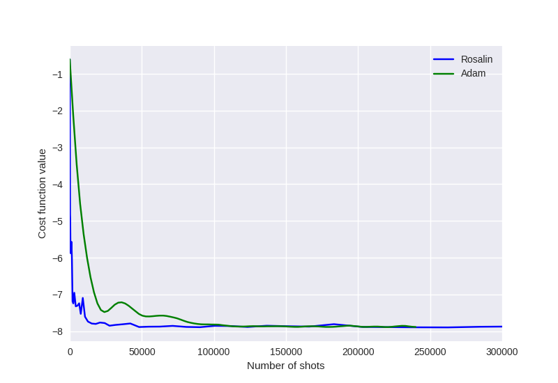
The Rosalin optimizer performs significantly better than the Adam optimizer, approaching the ground state energy of the Hamiltonian with strikingly fewer shots.

While beyond the scope of this demonstration, the Rosalin optimizer can be modified in various other ways; for instance, by incorporating weighted hybrid sampling (which distributes some shots deterministically, with the remainder done randomly), or by adapting the variant iCANS2 optimizer. Download this demonstration from the sidebar 👉 and give it a go! ⚛️

References

1(1,2,3,4)

Andrew Arrasmith, Lukasz Cincio, Rolando D. Somma, and Patrick J. Coles. “Operator Sampling for Shot-frugal Optimization in Variational Algorithms.” arXiv:2004.06252 (2020).

2

James Stokes, Josh Izaac, Nathan Killoran, and Giuseppe Carleo. “Quantum Natural Gradient.” arXiv:1909.02108 (2019).

3

Ryan Sweke, Frederik Wilde, Johannes Jakob Meyer, Maria Schuld, Paul K. Fährmann, Barthélémy Meynard-Piganeau, and Jens Eisert. “Stochastic gradient descent for hybrid quantum-classical optimization.” arXiv:1910.01155 (2019).

4(1,2)

Jonas M. Kübler, Andrew Arrasmith, Lukasz Cincio, and Patrick J. Coles. “An Adaptive Optimizer for Measurement-Frugal Variational Algorithms.” Quantum 4, 263 (2020).

About the author

Josh Izaac

Josh is a theoretical physicist, software tinkerer, and occasional baker. At Xanadu, he contributes to the development and growth of Xanadu’s open-source quantum software products.

demos/tutorial_rosalin

 

Download Python script

 

Download Notebook

 

View on GitHub